NAOJ GW Elog Logbook 3.2

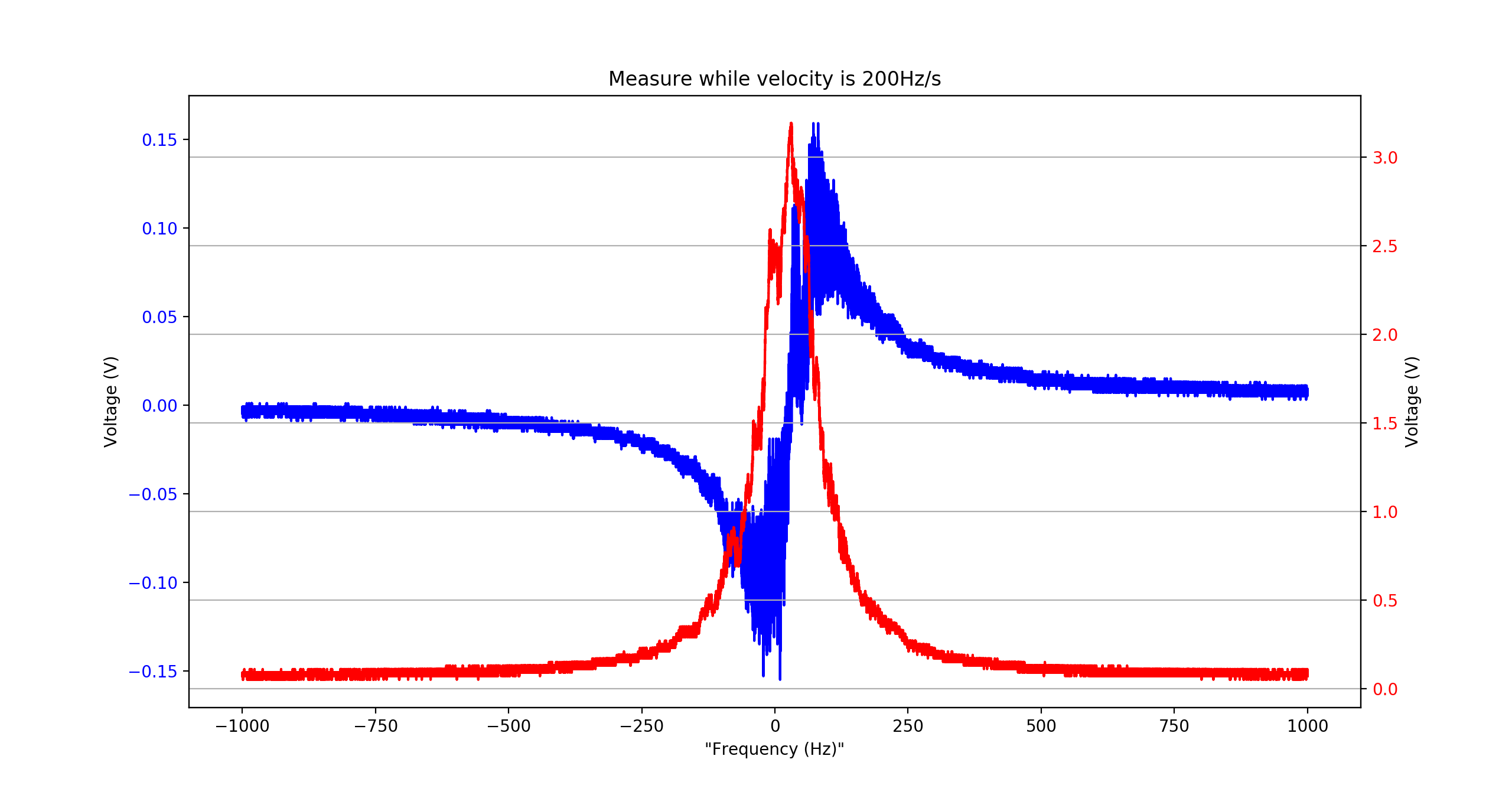
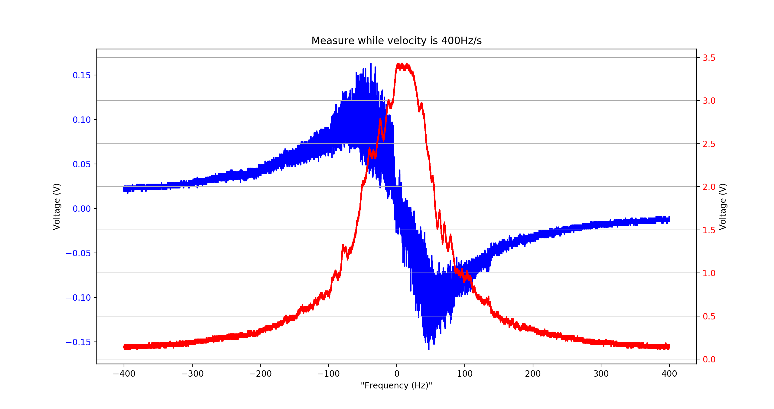
We measured the cavity bandwidth and error signal for IR with three different velocity of frequency scan. In this case, we can give a reasonable estimation of the calibration factor of IR. The result is 180.7 +/-5 Hz/V. We didn't consider error of invidual measurement, the standard deviation only comes from these three measurements results.
| velocity | bandwith | calibration |
| 200Hz/s | 106Hz | 176Hz/V |
| 400Hz/s | 112Hz | 186Hz/V |
| 80Hz/s | 108Hz | 180Hz/V |
For a better parameter estimation, we will fit these measurment result.

As pointed out by Matteo B., the spectrum in the entry693 was not correct. After some investigation, we found the problem comes from the conversion of .DAT file.
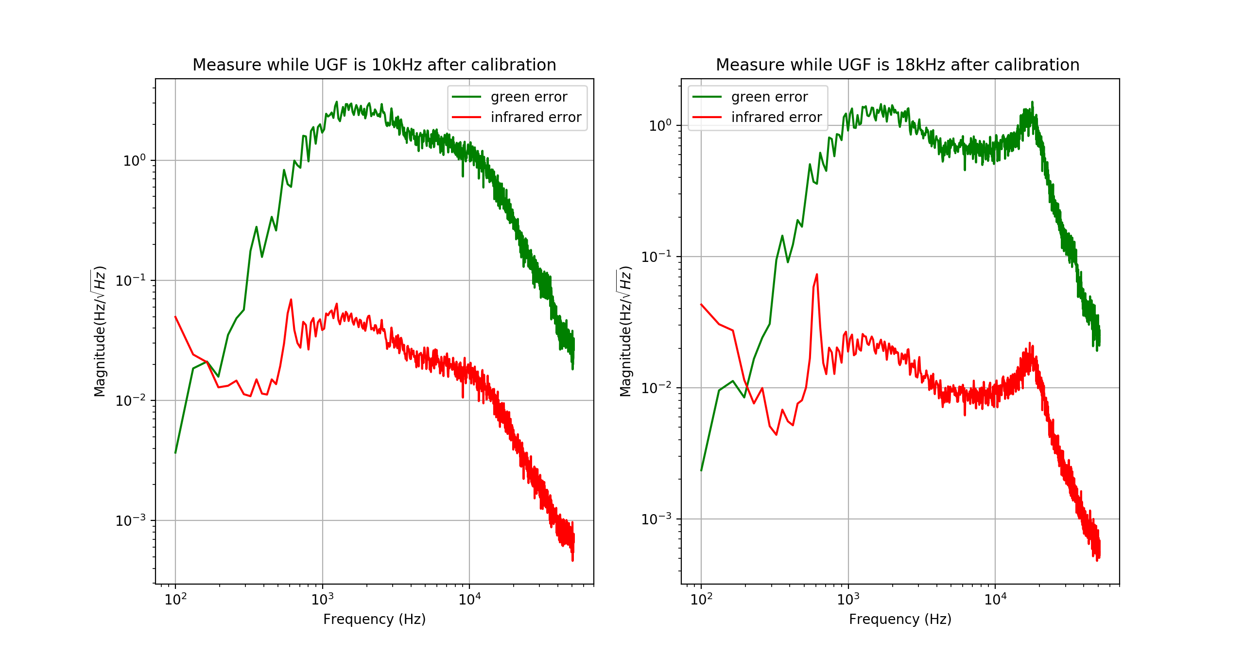
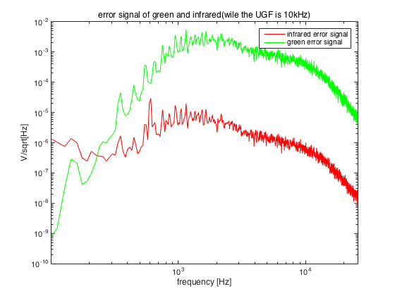
After solving this problem, we compared the spectrum of green and infrared error signal, taken with different value of loop's UGF(10kHz and 18kHz). Now we are using UGF as 18kHz.
In the attached plot there are calibrated spectrum. The calibration factor we are using for green is 385Hz/V, for infrared is 180Hz/V.
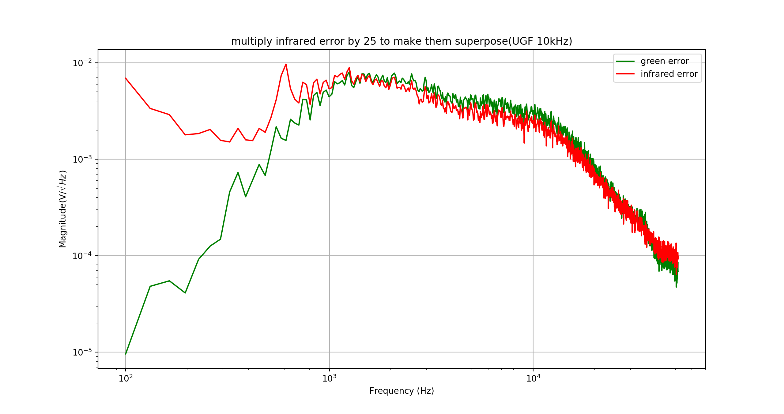
We also multiplied a factor to make green and infrared superpose. We can see from the attached plot that green and infrared have the same trend at high frequency. This is in agreement with the fact that after 1.4kHz we should also see the effect of the green cavity pole.
The .txt files attached are not calibrated.


Participants: Eleonora, Matteo L, Yuefan
We did a preliminary try to implement the dithering technique to keep the beam direction aligned with the cavity axis by acting on BS pitch and yaw.
We started with yaw:
1) We inject a sine perturbation in BS yaw with frequency 10 Hz and amplitude 3mV.
2) We acquired the transmitter green power in labview using one of the spare channel of the "telescope" ADC board.
3) We demodulated it by multipling it for a sine with the same frenquency and filtered it with a lowpass (butterworth 4th order, cutoff frequency 1 Hz)
4) We filtered the error signal with another lowpass (butterworth 1th order with cut off frequency at 0.01 Hz and adjustable gain).
5) We summed the correction signal to the "manual offset" in the yaw local control loop which is usually set by hand during the manual alignement procedure.
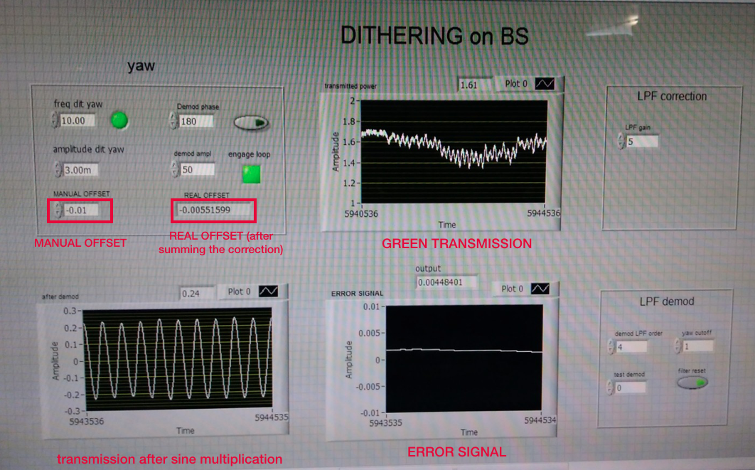
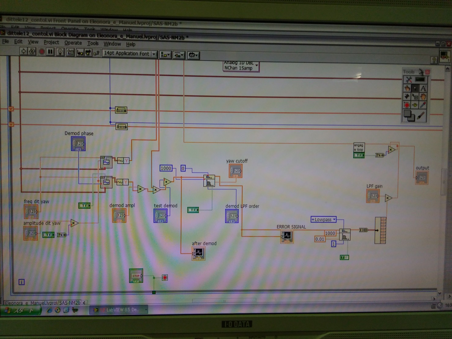
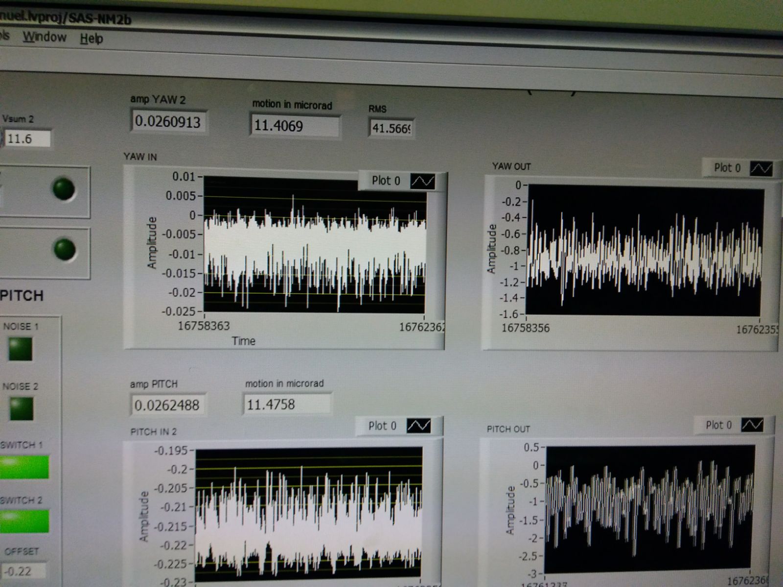
In Pic. 1 there is an "explained" scheme of the labview frontpanel, in Pic. 2 there is the block diagram of the vi.
The attached video shows the effect of the loop when we change the manual offset of BS yaw. The starting position is 0.02. We change it to 0.01 and to 0.
(See Pic.1 for a reference of the different controls and graph shown)
It seems that the loop is somehow able to bring back the offset to a position which makes the transmitted power less sensitive to the modulation. We need to check the long term performances and implement the same loop on the other degree of freedom.
DEMODULATION PHASE ISSUE
We tried to adjust the demodulation frequency by adding a tunable phase difference between the signal sent to the BS and the one used for the demodulation. With the loop open, we tried to change the demodulation phase in order to maximize the error signal but we couldn't see any change. We suspect that there is a problem with the reset of the subvi used to generate the sine wave. We might have found a solution that we will try soon. Anyway for the moment the demodulation phase is not optimized.
Link to the video in mp4 format.
https://drive.google.com/file/d/178Y6unT0S023VQCVl7pdYEdYgbTta22U/view?usp=sharing

Today, We try to use a way to measure the decay time of our filter cavity. The way is to cut the incident laser mechanically. By taking the data of oscilloscope, I used this function to fit
y=np.exp(-t/a1)+np.exp(-t/a2)
The reason I use this function is we have two decay mechanisms. One is mechanical cutting, the other is cavity decaying. The fitting result is a1=0.000326, a2=0.0025. This means the cutting time is 0.000326s and cavity decay is 0.0025s.(See attached Fig 1)

I've compared the error signals measured in the entry 690 with the new ones. There is something strange: now the error signal for the IR is 10 times smaller than before.

PARTICIPANTS: Yuhang, Yuefan, Eleonora
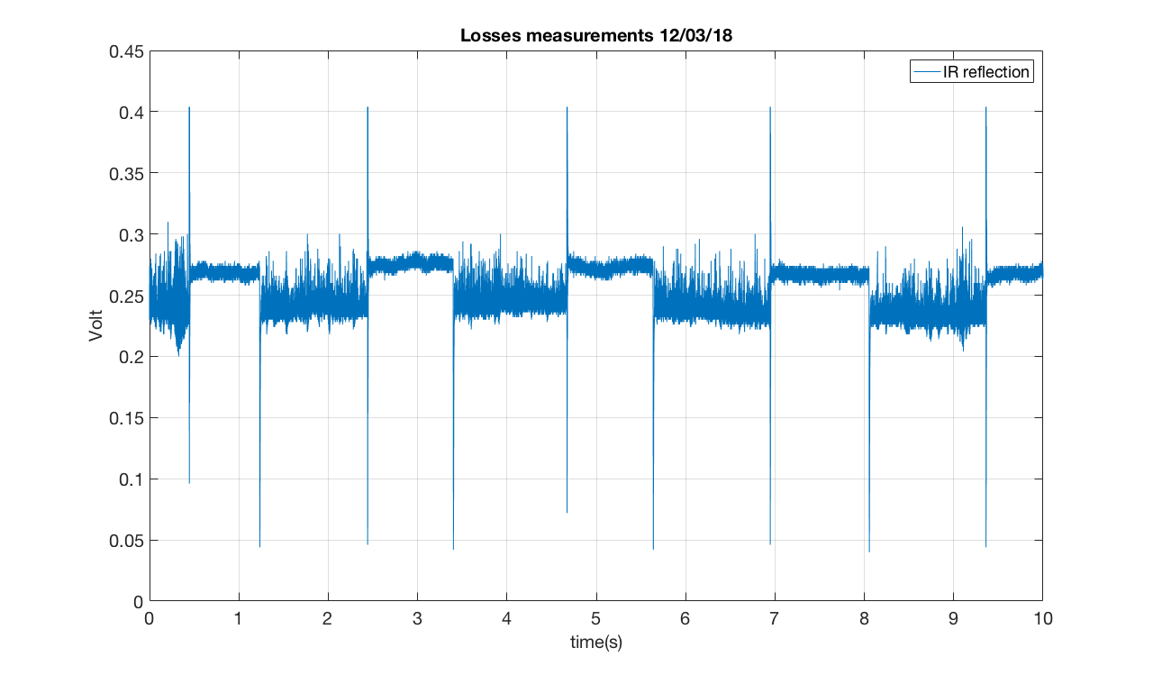
In the past days we have monitored the cavity round trip losses. We computed them from the cavity reflectivity with the tecniques described here.
In the actual setup the losses are measured using the IR reflected beam, sensend by a TAMA fotodiode. The reflected beam is filtered whith a bandpass filter in order to get rid of the residual green and it is focused on the photodiode using a 2 inch lens with f = 30 mm. (See first attachment for the setup scheme)
With this setup we have found that the reflectivity (ratio between reflected power in lock and out of lock) changes from day to day and takes values between 0.88% and 0.82%. It corresponds to a variation in the RTL between 40 ppm and 75 ppm.
The change can be due to the different alignment condition (the beams impinges on different points of the mirror which scatter differently) and/or to some other factor affecting the measurement and not yet understood.
In the attached plotes there are some measurments from the last days. Unfortunately not all the measurements from which we deduce the RTL variation reported before have been recorded.
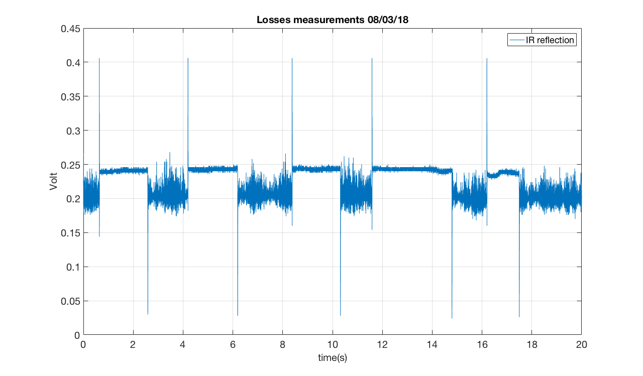
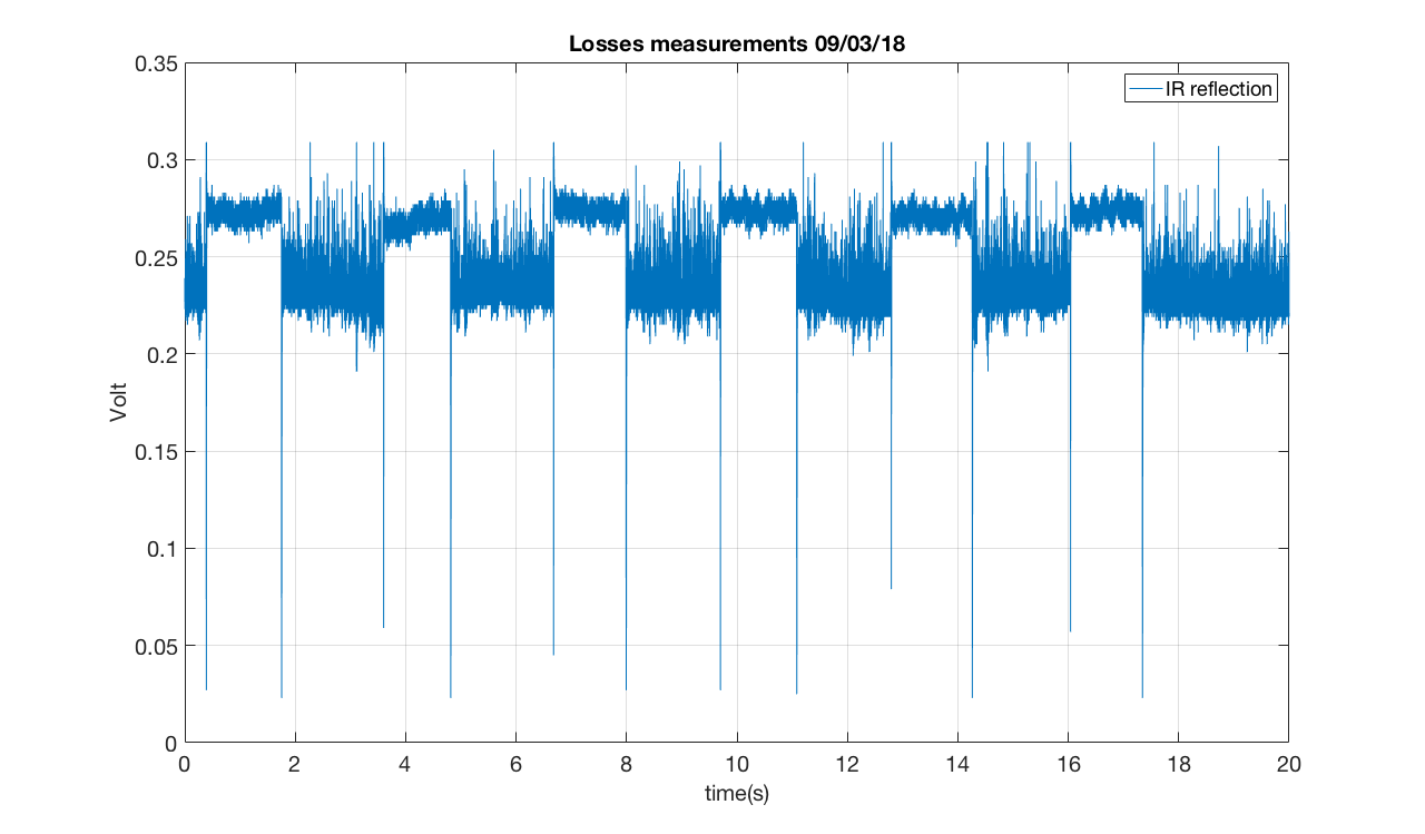

In order to increase the statistic yesterday we repeated the measurement of the round trip losses, with the lock unlock technique.
Since we did it in two different moments of the day the alignement conditions were likely to be different.
| reflectivity | losses | |
| #1 | 0.87±0.02 | 50±13 |
| #2 | 0.80±0.03 | 81±16 |
The reflectivity has been computed by taking the mean of the time series between a lock and an unlock period. The error is computed as the progagation of the standard deviation of these two set of data.
We estimated that 7% of the input light does not couple into the cavity.
New did a new measurement of RTL with lock/unlock.
Reflectivity 84% +/- 2% => Losses 63±12 ppm
We considered that 7% of the input light is not coupled into the cavity.
Loss measurement 28/03/18
Reflectivity: 89%+/- 2.5% => Losses: 44 +/- 12 ppm
Mismatching/misalignement considered in the estimation: 11% (worse than usual)
Yesterday, we did some characterization of our filter cavity.
1. Open Loop Transfer Function: The unity gain frequency is 10kHz and the phase margin is 39 degree. Actually this is not the practical case, we changed the gain of our loop. And we suspected this is because of the increase of circulating power.(Fig 1)
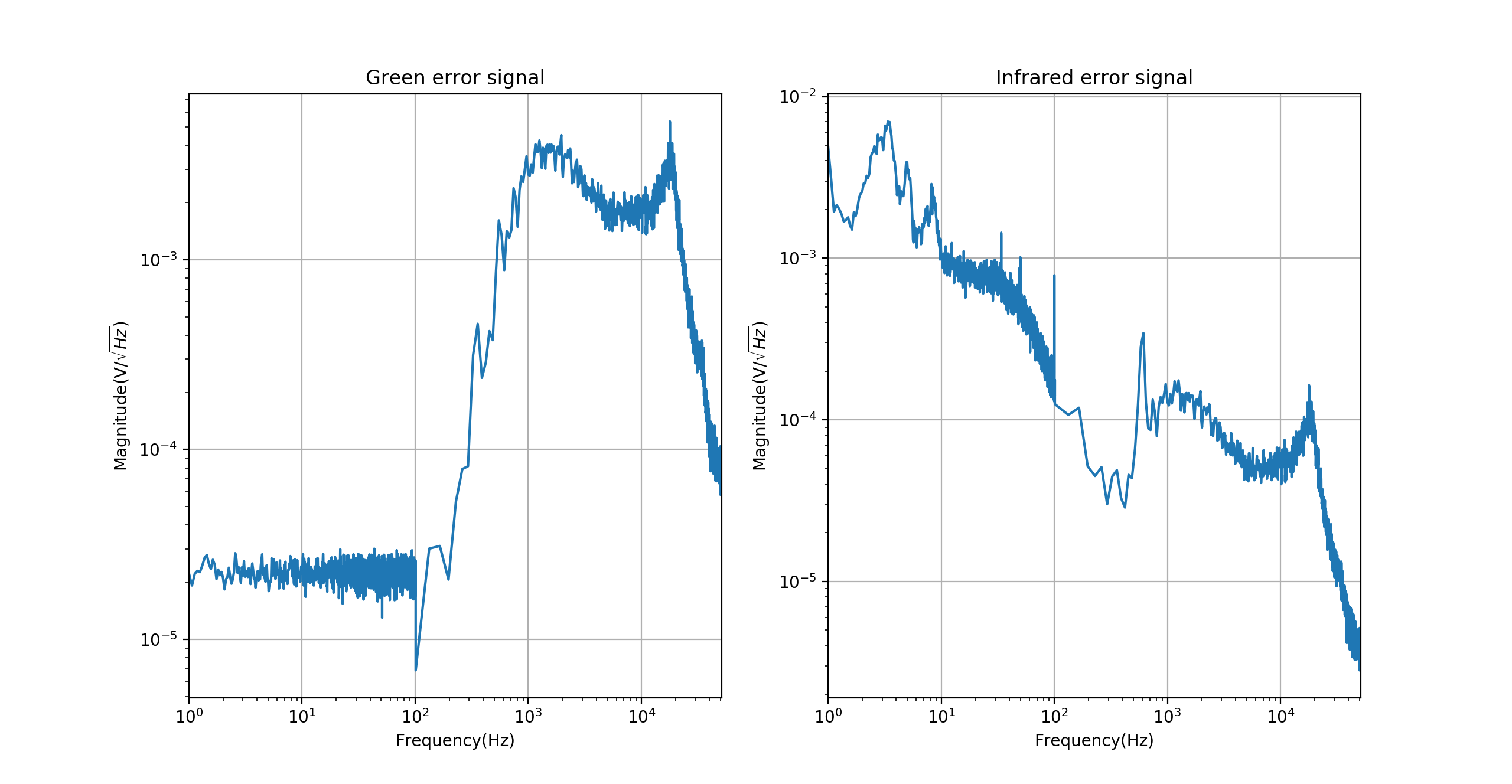
2. Calibration: We measured the calibration of green and infrared again. The calibration factor is similar with before.(Fig 2)
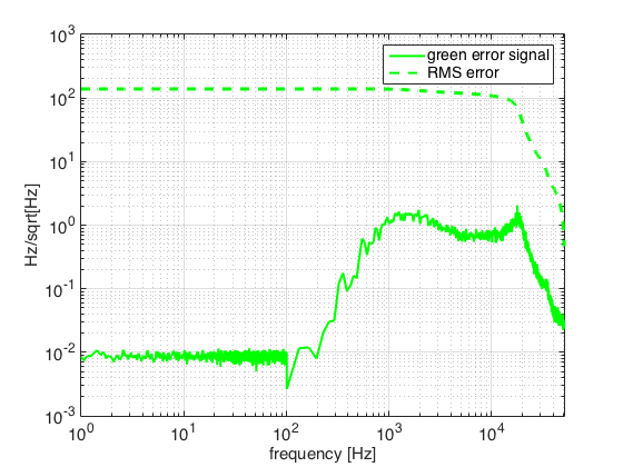
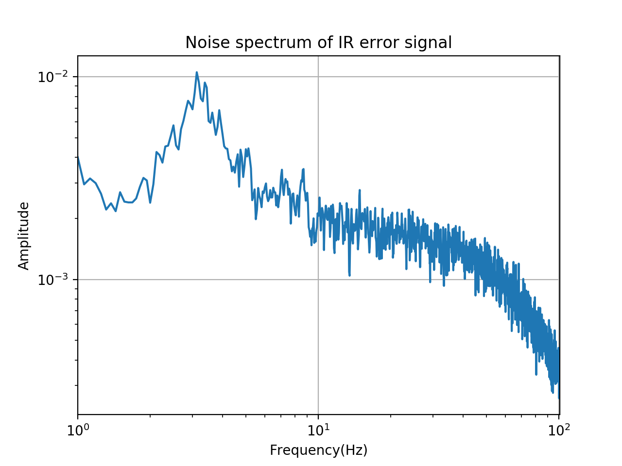
3. Error signal noise spectrum: We plot out the direct measurement and calibrated one together.(Fig 3 and 4)
You can use the data attached. They are not calibrated.
ger25k6 is green error signal with highest frequency 25600Hz(calibration factor is 2.6e-3V/Hz).
ier25k6 is infrared error signal with highest frequency 25600Hz(calibration factor is 6.3e-3V/Hz).
ol51k2 is open loop transfer function with highest frequency 51200Hz.


I've compared the error signals measured in the entry 690 with the new ones. There is something strange: now the error signal for the IR is 10 times smaller than before.
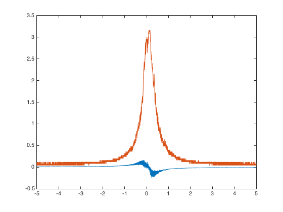
In order to reproduce the "Pacman" shape seen in the reflected beam (see #entry 687), I have made a simulation of the cavity using the FFT code OSCAR.
https://fr.mathworks.com/matlabcentral/fileexchange/20607-oscar?requestedDomain=true
The shape is more or less reproduced with a mismatching of 4% and a misalignemnt of 5microrad of the end mirror.
I attach the plot of the fields and the script used (it needs the code OSCAR to be used), which can be useful also for other applications.

I also attach the txt file here. It has not been calibrated yet. The calibration factor I used here is 2.6e-3 V/Hz(for green), 170Hz/V(for infrared).
Yesterday at some point the lock was disturbed by some spikes affecting the BS local control signals. The problem could be temporarily solved by switching off and on the laser.
In the past weeks we observed in two ocassions glitches affecting the error signals of the end mirror local controls.
When the control loops are open, the glitches look like "jumps", affecting simultaneusly both pitch and yaw.
They are quite frequent and in most of the cases they cause the unlock of the cavity. In both cases the problem was solved by switching off and on the ADC in the end room.
Participants: Yuhang, Yuefan, Tomura, Raffaele, Eleonora
In the past days we have worked in order to improve the IR alignment.
As a first thing we placed a camera on the optical bench to look at the IR reflected beam and we tried to maximized the trasmitted power while monitoring the shape of the reflected beam. According to our understanding, in reflection we should see the superposition of the resonant TEM 00 (dephased of 180 deg after it is reflected by the cavity) and the HOM due to misalignement/mismatching which are promplty reflected.
The procedure to align the cavity both for green and IR is the following:
1) Adjust BS position to center the beam on the end mirror (reference on the end camera screen)
2) Align the cavity for the green beam by moving input and end mirror to maximize the transmitted power
3) Move the last two steering mirror for the IR on the bench to maximize IR trasmitted power
4) While aligning the IR we take care that it is always centered on the resonance by looking at the error signal and adjustig the AOM frequency to null its offset.
During in this activity we realized that the alignement improvement was limited by the position of the last IR steering mirror on the bench. So we have shifted it after carefully taking some references in order not to loose the alignment. After this change we were able to improve the IR transimitted power from about 2.5 up to more than 3.5 V
Currently in the best alignement condition we have about 1.8 V of transmitted power for the green and 3.8 for the IR.
The attached video shows the reflected and the trasmitted IR beam when we change the alignment condition in pitch and yaw by moving the steering mirror on the bench. In the case of strong misalignement the presence of first order modes becomes evident. Anyway also in the best aligment condition (about 95 %) there is still a small black dot in reflection.
The oscilloscope in the video shows the transmitted power (yellow line) and the IR error signal (blue line).
After this change in the alignement we have verified that the IR beam in refection was not touching a side of the viewport. (See entry #659 related to this issue )
In order to calibrate the IR error signal we have scanned the resonance by adding a modulation to the AOM around the resonance driving frequency.
We choose a triangular wave, with period 50 mHz and amplitude of 2 kHz (which corresponds to 1 kHz for the IR). This means that the resonance is crossed with a constant speed of of 200 Hz/s.
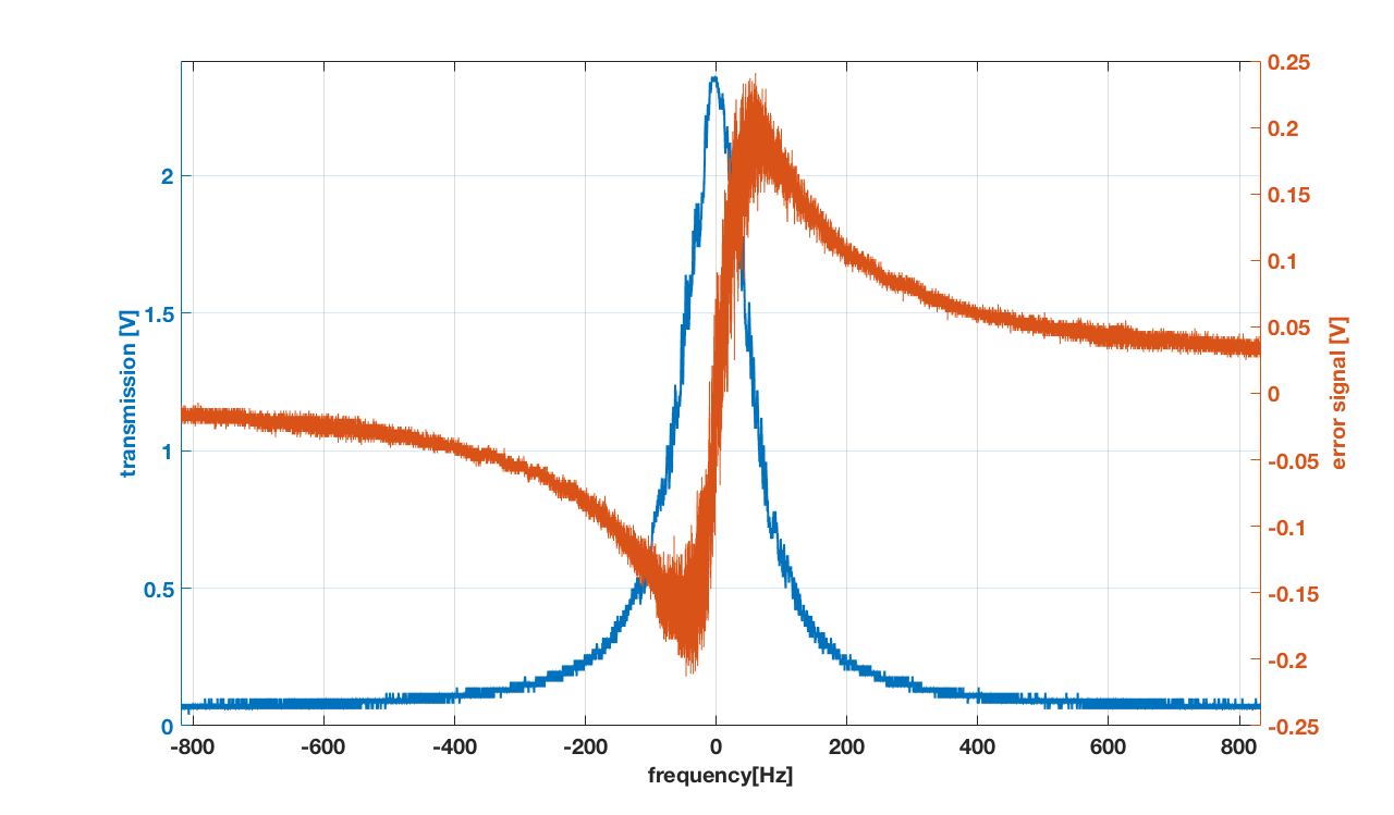
In the first attached picture, the IR transmission and the error signal are shown during a crossing of the resonance. The x axis has been calibrated in Hz using the computation reported before.
The FWHM of the trasmission is about 116 +/- 4 Hz, corresponding to a finesse of 4310 +/- 150, which is comparable with the design and the previous measurements.
The correspondig PDH has been used to calibrate the IR error signal, finding a value of about 170 +/- 20 Hz/V
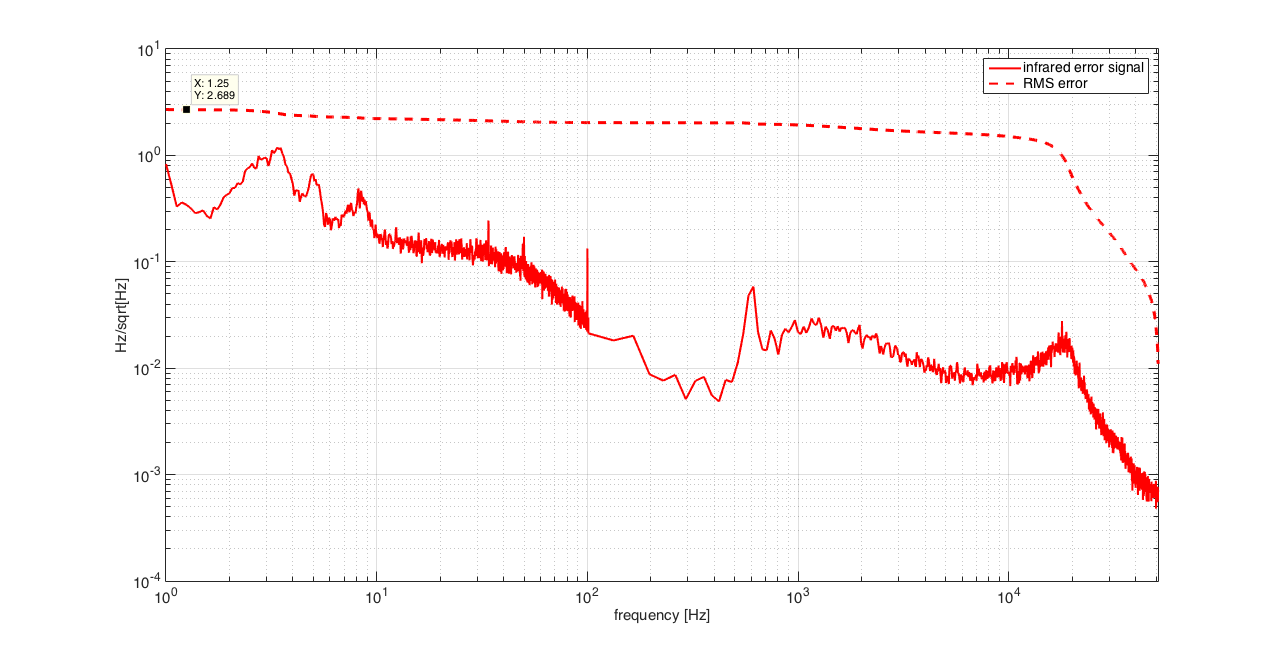
The second plot shows the calibrated IR error signal, when the cavity is on resonance. The RMS is about 4.4 +/- 0.5 Hz.
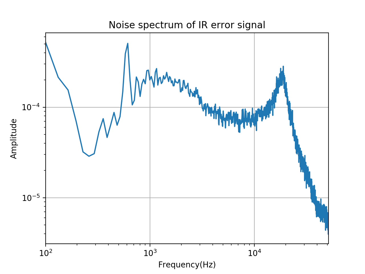
In the third plot, I have merged and calibrated the spectra of the error signal recorded with the spectrum analyzer in two different frequency regions (from 1Hz to 100 Hz and from 100 to 51kHz) and I have computed and plotted the rms. As expected it is in agreement with that found from the time series.
According to the plot, the high frequency (above 100 Hz) seems to contribute with 3.5 Hz to the total rms. The remaing (about 1 Hz) is accumulated below. The contribution of the suspension resonances in the region from 1 to 10 Hz is visible and seems to be about 0.5 Hz.
The origin of the peak at 12 kHz and the quite complex shape of the signal are not very clear to me.
Next step will be to comprare this spectrum with that of the green error signal in order to investigate the role played by the IR pole.


After changing the photodiode and the mixer box, we can get a proper error signal now. From this error signal, we can get many useful information.Including:
1. We can use this error signal to tell if our alignment or frequency setting is making the TEM00 on resonance. That means if TEM00 is on resonance, the IR error signal is properly around zero. This is a very good standard to adjust our IR beam.
2. We can also use it to evaluate the locking accuracy.
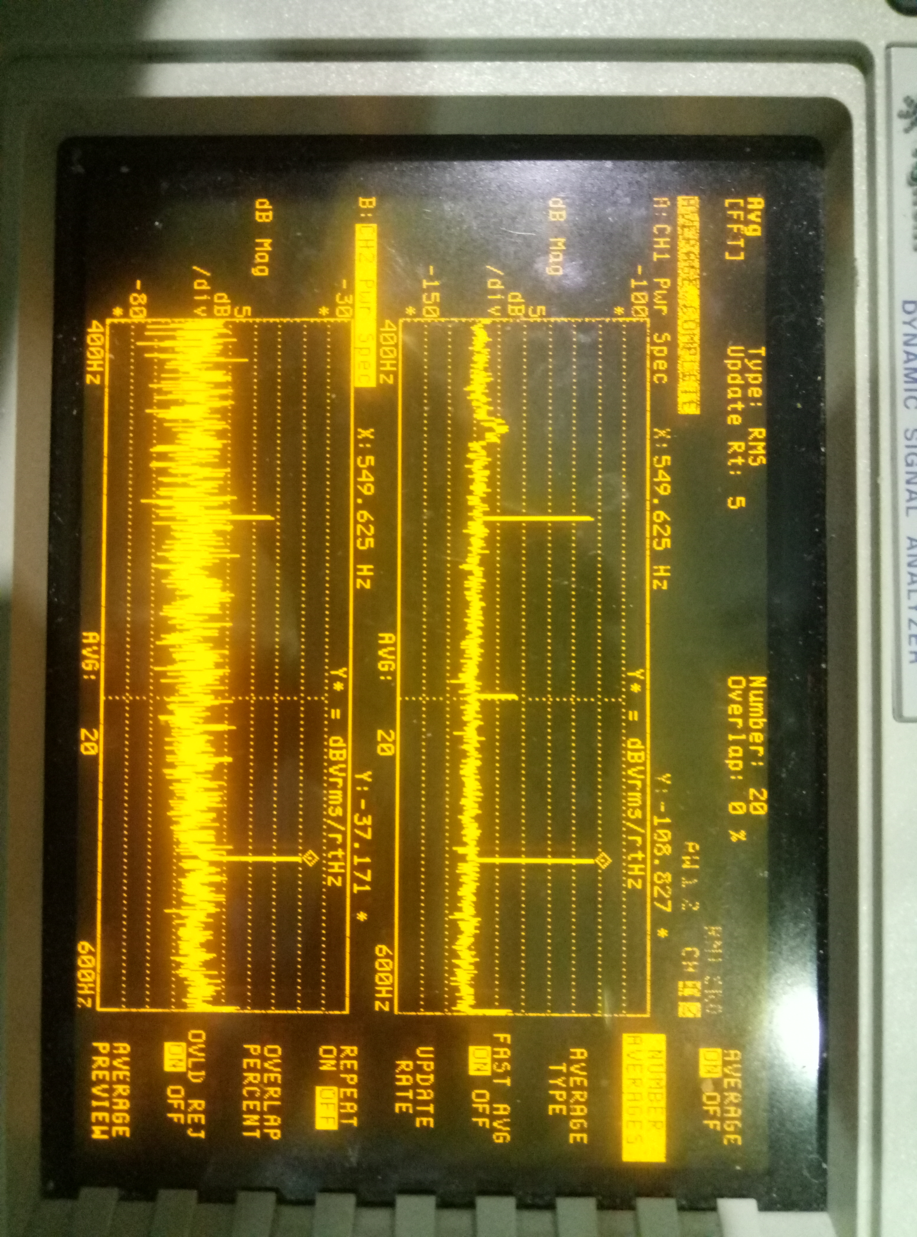
3. By measuring the noise spectrum of this error signal, we can know it is correcting which frequency mostly. I attached this measurement as picture one and two. We can see that 3Hz, 500Hz and 20000Hz are the main three peak frequency.
The data corresponding to this picture you can find here
https://drive.google.com/drive/folders/1J2PmI-GSoQ-BA4gE1VS5wI8wLsPURzoF?usp=sharing
In order to calibrate the IR error signal we have scanned the resonance by adding a modulation to the AOM around the resonance driving frequency.
We choose a triangular wave, with period 50 mHz and amplitude of 2 kHz (which corresponds to 1 kHz for the IR). This means that the resonance is crossed with a constant speed of of 200 Hz/s.
In the first attached picture, the IR transmission and the error signal are shown during a crossing of the resonance. The x axis has been calibrated in Hz using the computation reported before.
The FWHM of the trasmission is about 116 +/- 4 Hz, corresponding to a finesse of 4310 +/- 150, which is comparable with the design and the previous measurements.
The correspondig PDH has been used to calibrate the IR error signal, finding a value of about 170 +/- 20 Hz/V
The second plot shows the calibrated IR error signal, when the cavity is on resonance. The RMS is about 4.4 +/- 0.5 Hz.
In the third plot, I have merged and calibrated the spectra of the error signal recorded with the spectrum analyzer in two different frequency regions (from 1Hz to 100 Hz and from 100 to 51kHz) and I have computed and plotted the rms. As expected it is in agreement with that found from the time series.
According to the plot, the high frequency (above 100 Hz) seems to contribute with 3.5 Hz to the total rms. The remaing (about 1 Hz) is accumulated below. The contribution of the suspension resonances in the region from 1 to 10 Hz is visible and seems to be about 0.5 Hz.
The origin of the peak at 12 kHz and the quite complex shape of the signal are not very clear to me.
Next step will be to comprare this spectrum with that of the green error signal in order to investigate the role played by the IR pole.
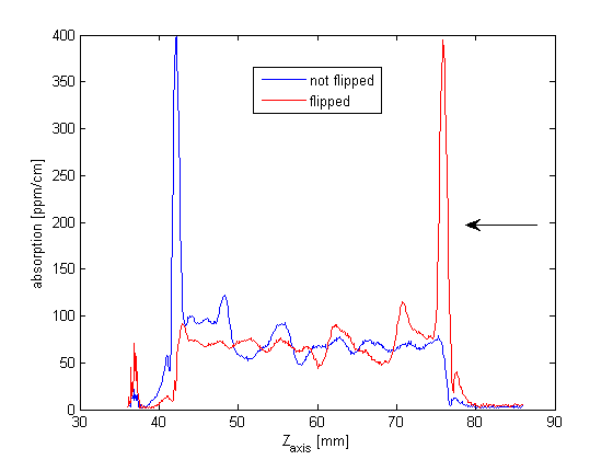
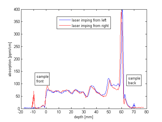
There was an alignment issue to be checked:
The pump and the probe laser inside a thick material are subject to the Snell's law.
Since the probe has a non-zero incidence angle, the crossing point changes position inside the material according to how much material the beams have traveled in before the crossing point.
If the beams are not perfectly horizontal and well aligned the car be an asymmetry on the absorption signal if the beams imping on one surface or on the other one.
To check this, I measured a scan at the center of the sample from one side, and I flipped the sample to do the same measurement from the other surface.
Result: the two plots overlap quite well.
The arrow in the first plot indicates where the beams come from
We have verified that the spikes oberved in the IR transmission, in the region above 10 kHz are prensent even if there is no light impingin on the photodiode. They are likely be due to electronics.
1. The installment of camera for IR reflection
Since we have received the filter to attenuate green beam, we tried to install the camera for IR reflection today. Since the power of IR is pretty high, we also used an OD filter(factor of 2) and a partly-reflected mirror to reduce the power. During the adjustment, we can see on the screen that there are two points. The small one is on the right and below side of the large one. Then we tried to change the angle of that partly-reflected mirror and accordingly the camera. At a certain point, we could make it a round point. We believed that that was a good angle.
Then we locked the cavity, this reflection of one point changes to two points.(See attached video 1) We thought that we were looking at the TEM10 mode. However, it should be the superposition of TEM00 and TEM01. According to our knowledge, this reflection can tell us the information of alignment. That means if it is the right reflection, we can use it to refine the cavity. Since we have already been around the best position, so we move the Input mirror around this position to check. What we could see is only these two points changed brighter and weaker one after another.(See attached video 2) Even when we tried to misalign the pitch of End mirror, we couldn't see the TEM01 mode on the screen.(See attached video 3)
Video Note: the interesting part of video are all around the end of video. You can find them by using the date 20180226. You can check them through this link. https://drive.google.com/drive/folders/1v7oSk0d6ONPN-NZTNcYjIuG0ip8XCZOn?usp=sharing
After checking all the things listed above, I felt gradually that it is not the right reflection. But we cannot figure out why we can see it. We need an expert and tomorrow Raffaele will come^_^
2. Attempt to acquire IR error signal
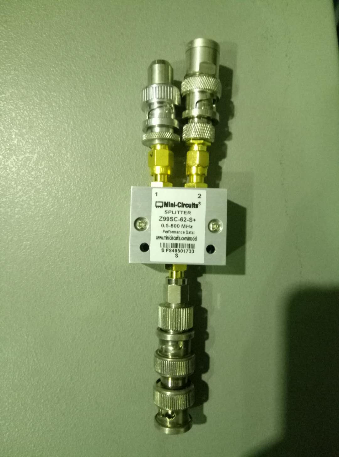
Due to the FWHM of IR is much more narrow than GREEN. The locking accuracy of IR needs to be evaluated by having the error signal directly. Owe to the EOM modulation for SHG, we have the modulation for infrared luckily. So we separate the output of its signal generator by using SMC-type connector(to avoid signal reflection see attached picture 1). We use the reflection from the cavity as RF signal.
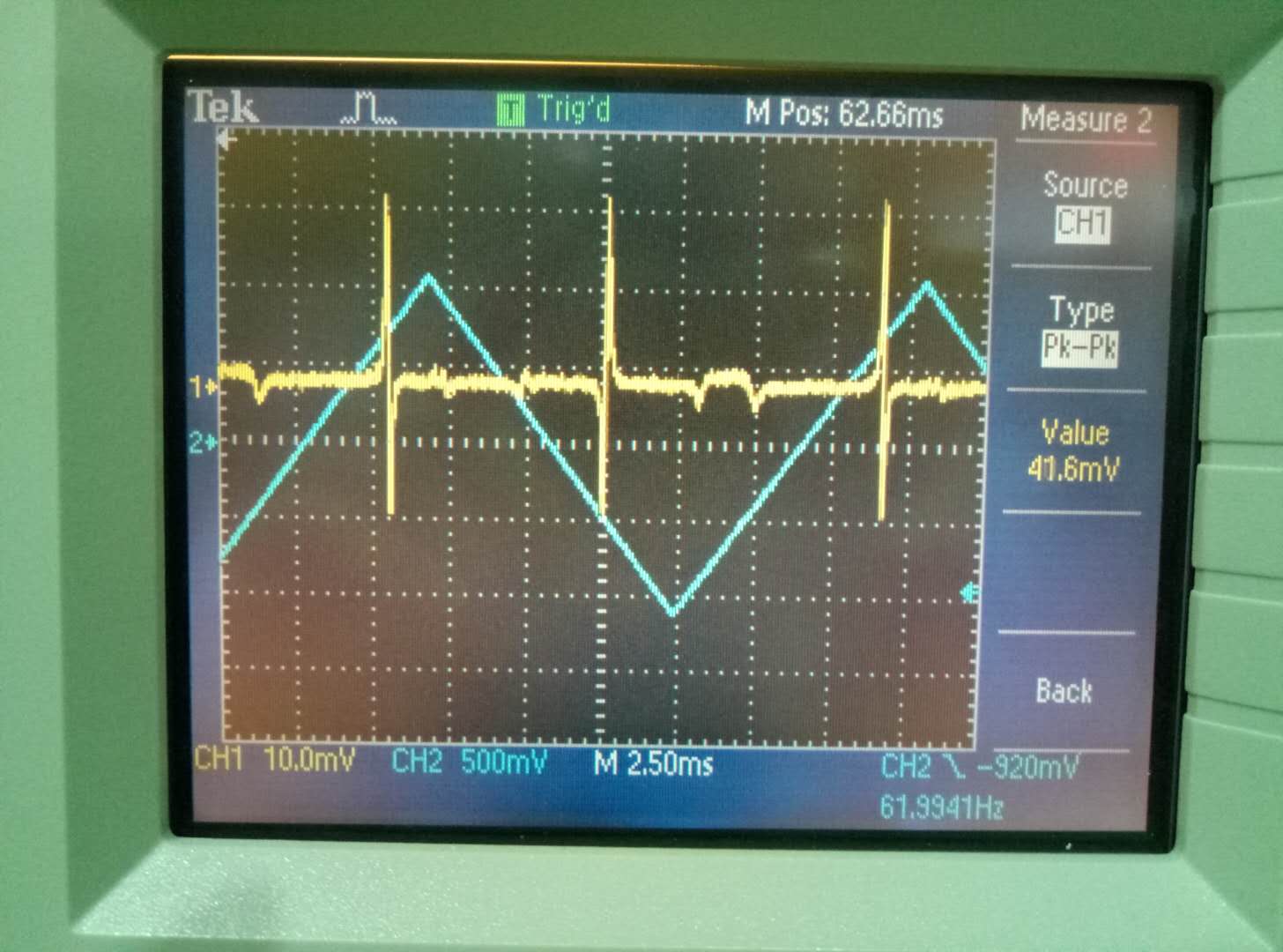
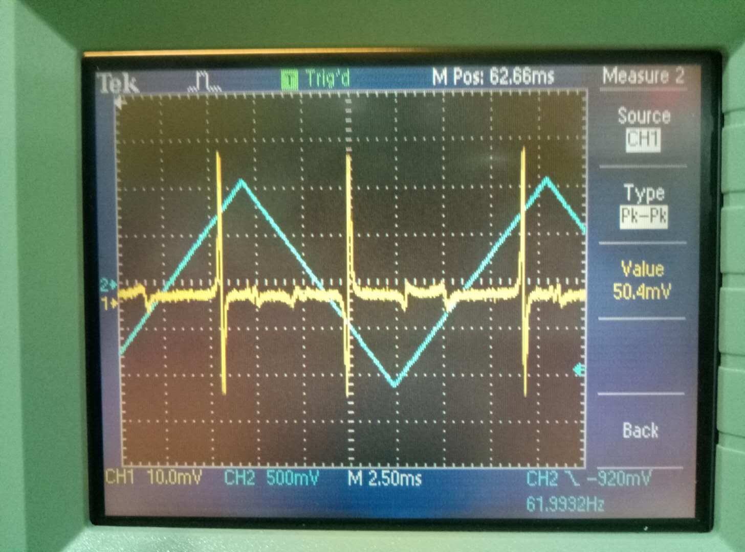
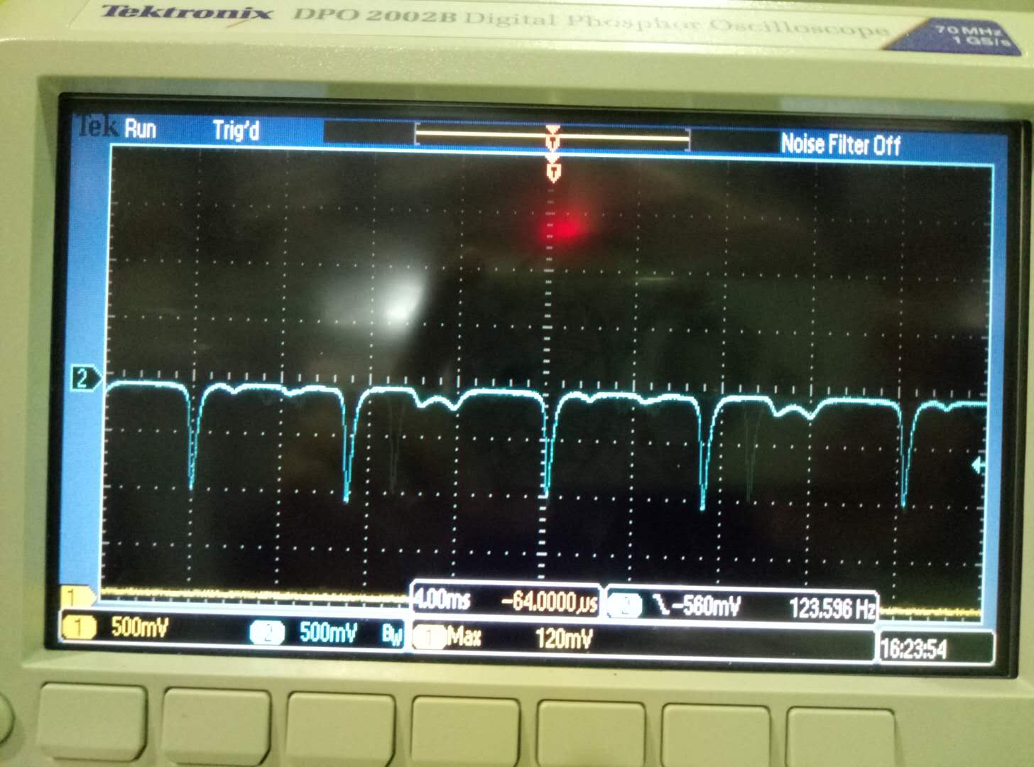
After separation, we succeeded in recovering the error signal for the SHG. By the way, we made this error signal pk-pk value larger than before.(See attached picture 2 and 3) Also we took the picture of different modes we got for SHG.(See attached picture 4)
For infrared error signal, we make the AOM modulate. That means the AOM driving frequency change around the best point with a certain frequency(It's like the ramp signal while we looking for the error signal). But we cannot find the error signal for IR.
For the fail of IR error signal, we found the bandwidth of IR reflection PD is not high enough. Now it is PDA36A(350-1100nm, 10MHz BW, 13mm**2), but our modulation is 15MHz. Certainly we cannot demodulate it. Besides, we also need to check if the demodulation board can work well tomorrow.
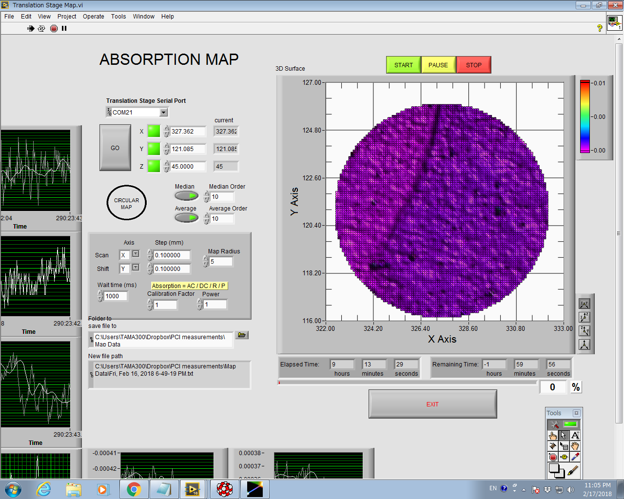
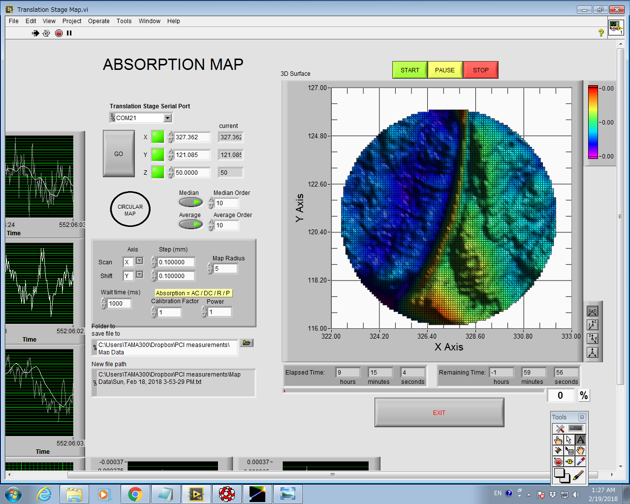
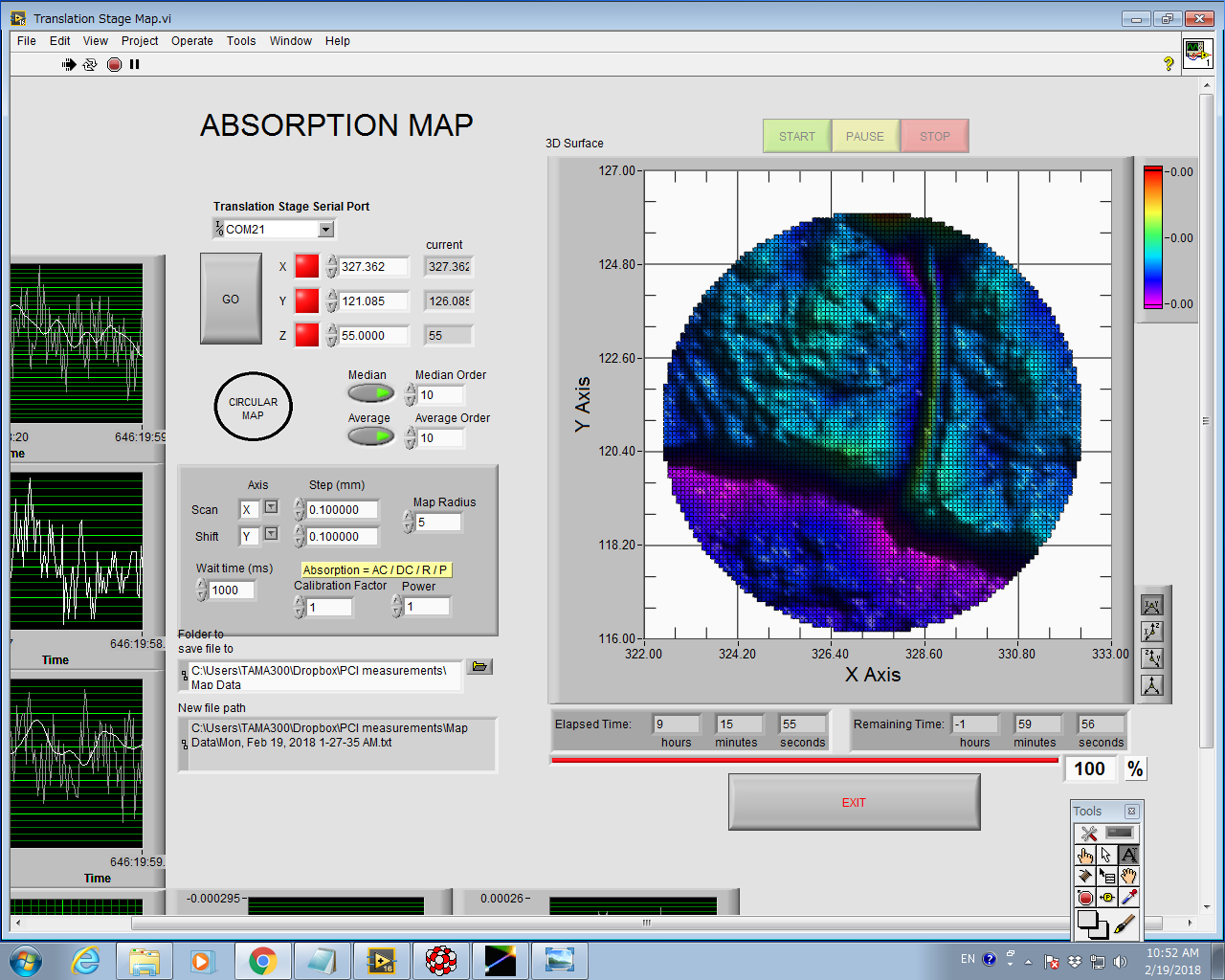
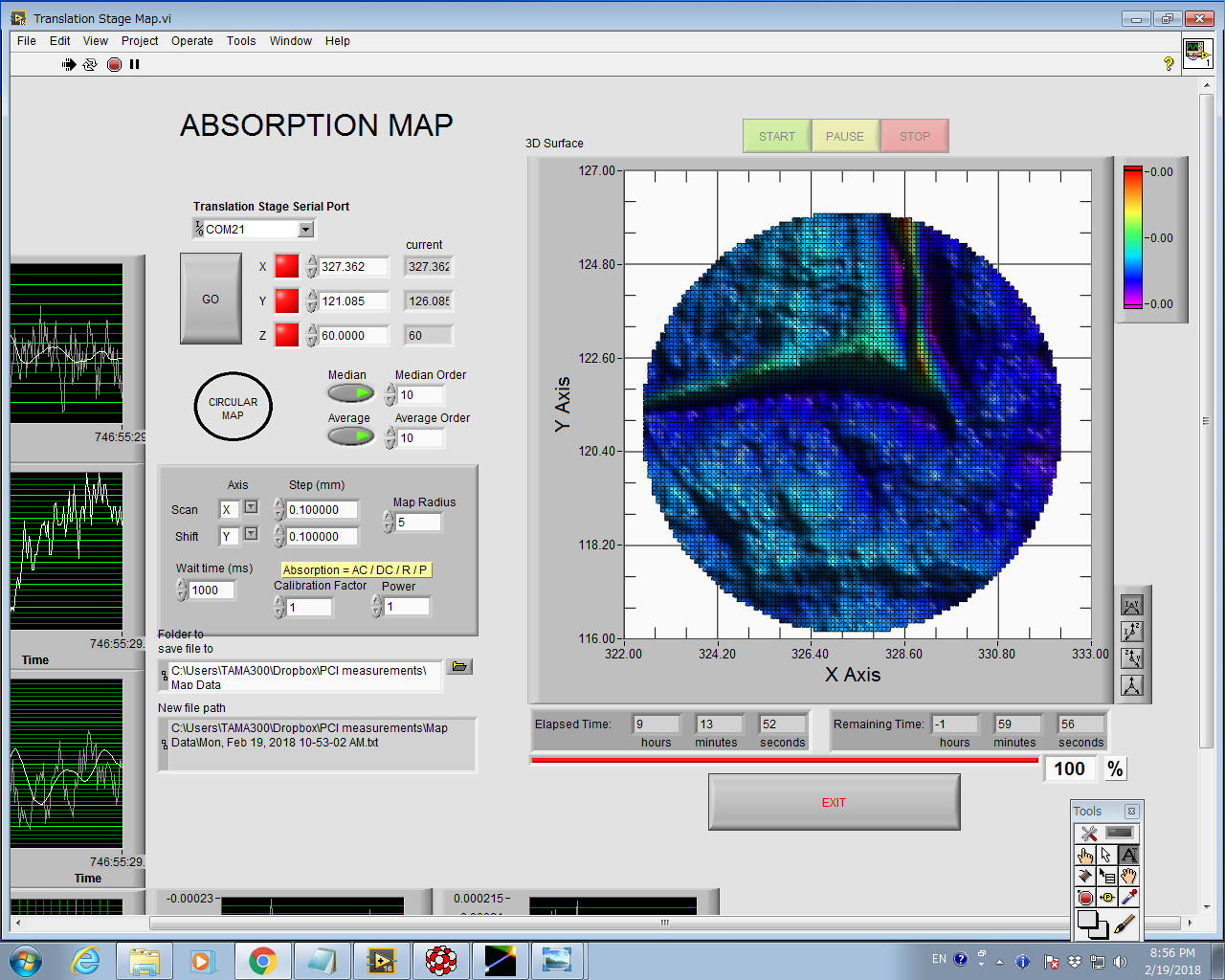
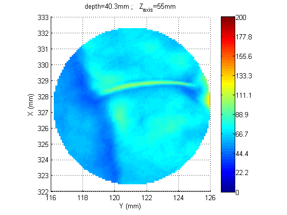
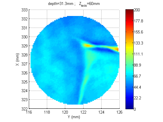
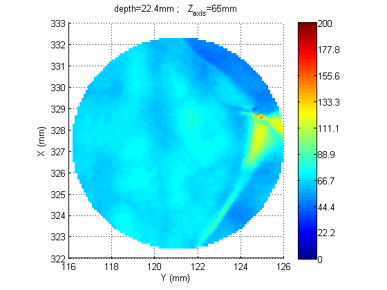
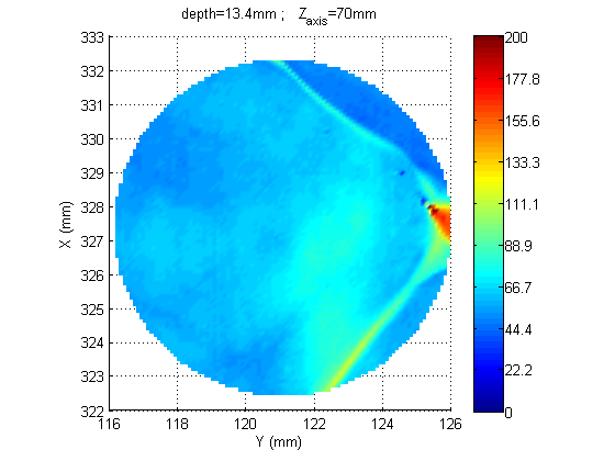
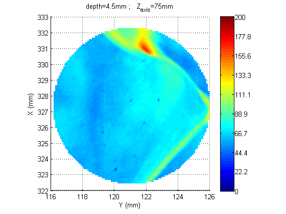
I characterized the absorption of the central part of the tama-sized sapphire substrate sample#2
Pump power 10W (after the chopper). Max laser current: 7.5A
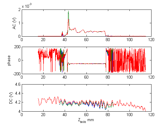
After aligning the system with the surface reference sample, and scanning the bulk reference sample for calibration (with power=30mW), I made a scan of the sapphire substrate.
Changing from the 3.6mm thick reference sample to the 60mm thick sapphire substrate we have to move backward the imaging unit by 24.9mm. Then recenter the probe on the PD maximizing the DC.
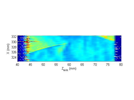
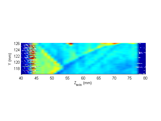
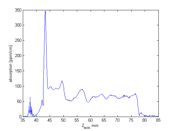
From the scan plot we can recognize the 2 surfaces of the sample (when the absorption signal drops to 0) and associate the translation stage Z coordinate to the sample coordinates. Indeed the apparent depth of the sample is different from the real one as explained in entry 242 , Since the sample is 60mm thick, it is convenient to define the sample Z coordinate to be 0 at the first surface and 60 at the second surface. On the translation stage reference system the first surface is at 44mm and the second surface is at 77.5mm. In other words, during a scan, the crossing point pump-probe travels in the sample about 1.8 times faster than the translation stage that mpoves the sample.
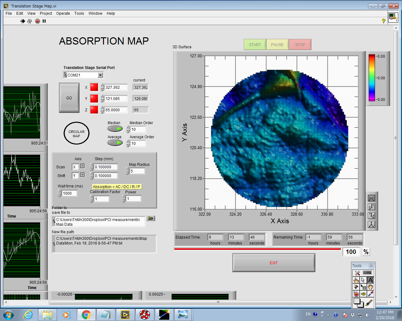
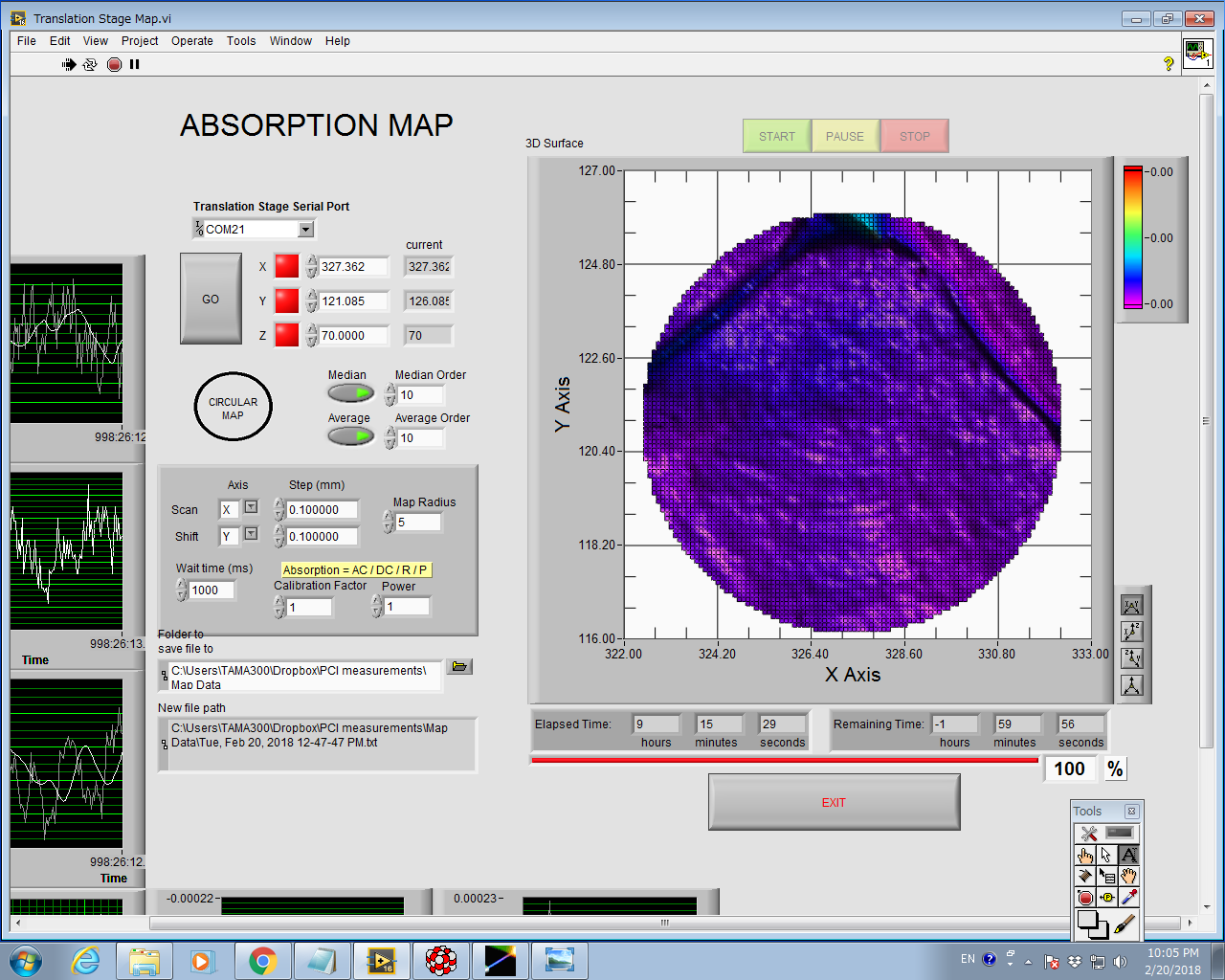
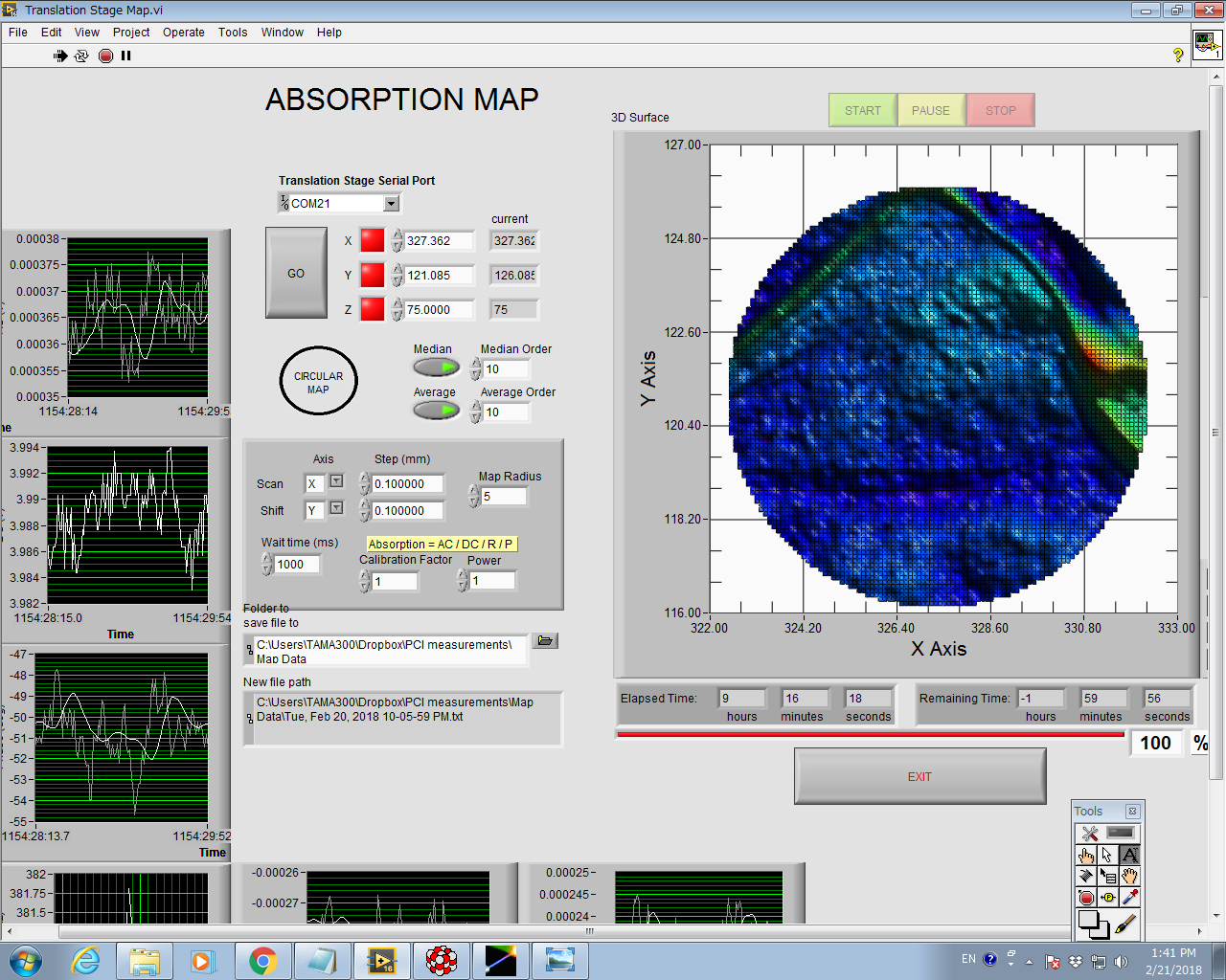
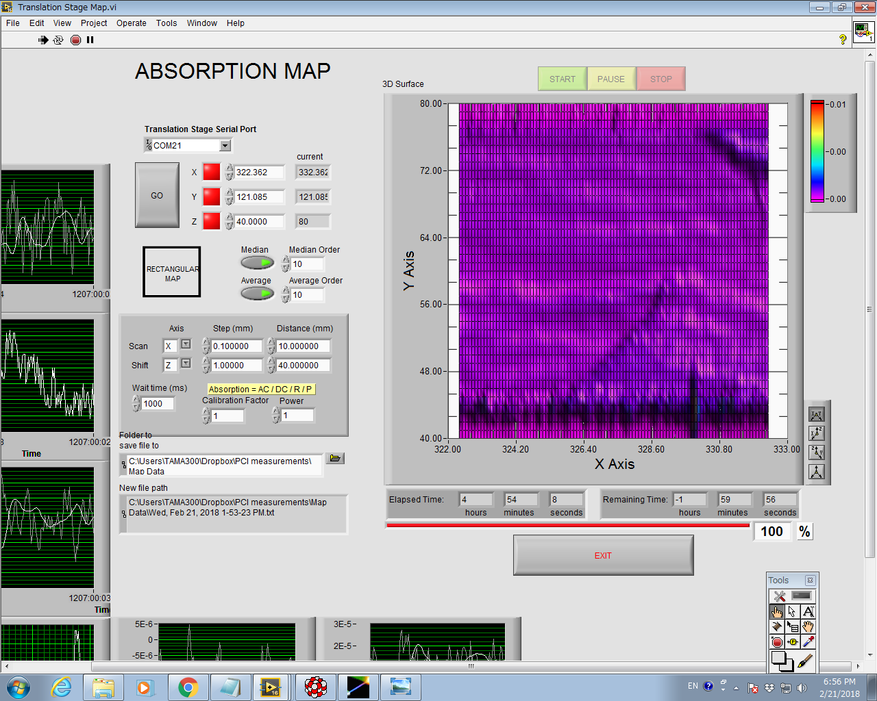
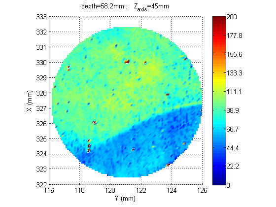
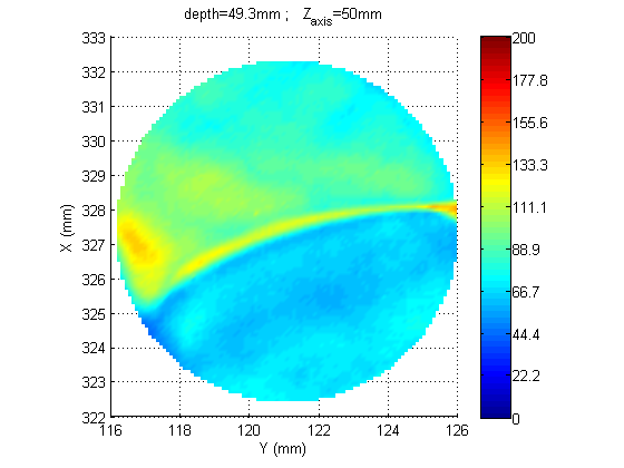
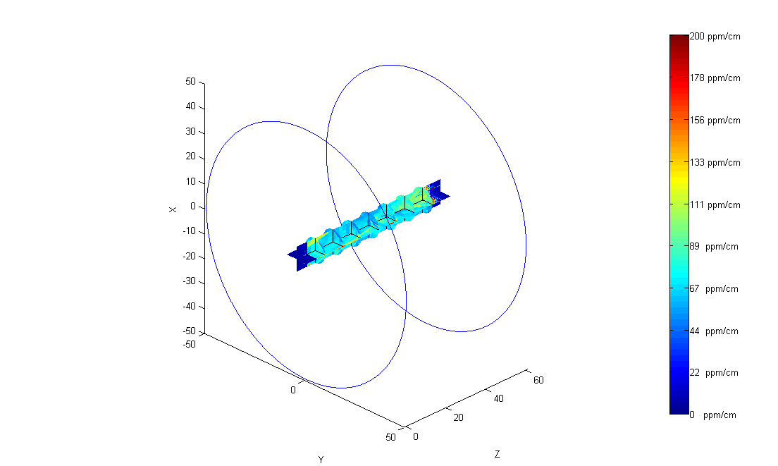
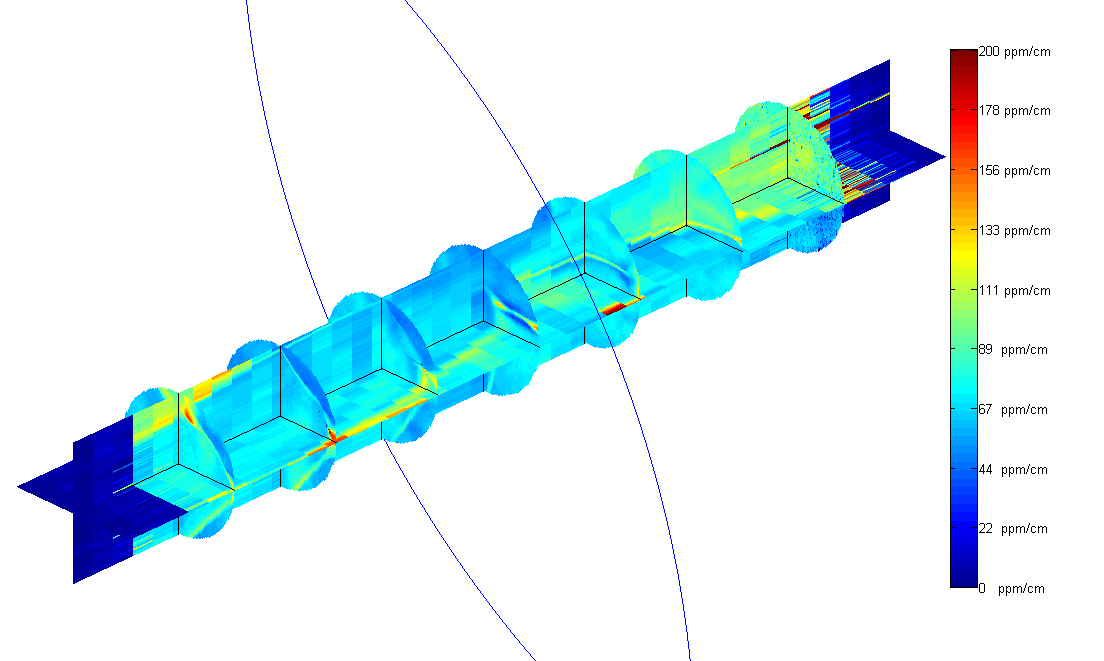
I made circular maps on the XY plane at several depths in the sample. Then 2 rectangular maps on the XZ and YZ planes. A 3d overview can summarize all the maps together in comparison with the sample size (drawn as 2 circles for the surfaces boundaries)
The circular maps resolution is 100um x 100um
The rectangular maps resolution is 100um x 1mm
the waiting time from one point to the next one is 1s, according to the average and median filters of order 10.
the color scale is up to 200ppm/cm to make the maps more readable and cover most of the color range. However, on the second surface of the sample, there are some absorption peaks up to 1400 ppm/cm which are probably due to some dirt on the surface or some polishing defects

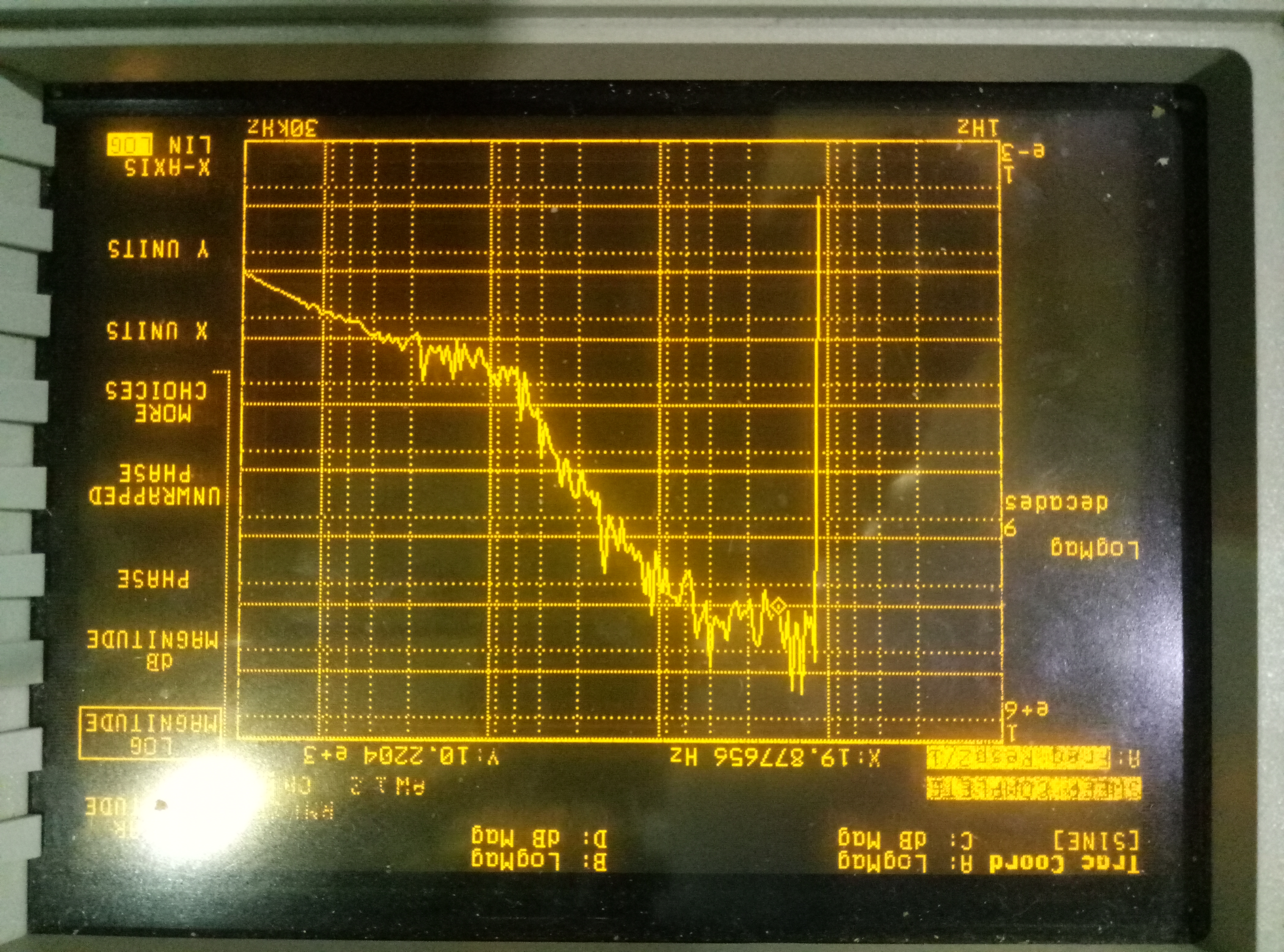
I made a mistake in entry672. The noise is injected in the position of CAVITY(G3). So we need to use open loop TF and G1,G2,G3 to calibrate this signal.
So I measured the open loop transfer function, it agrees with the simulation of Eleonora's thesis. For the measurement, the magnitude for 20Hz is about 10^4.(See picture 1)
Then using CH2*(open loop/(G1*G2*G3))=CH1. From this formula, we can do the calibration like entey672 again. This time, the result of calibration approximatly equals to the measurment.
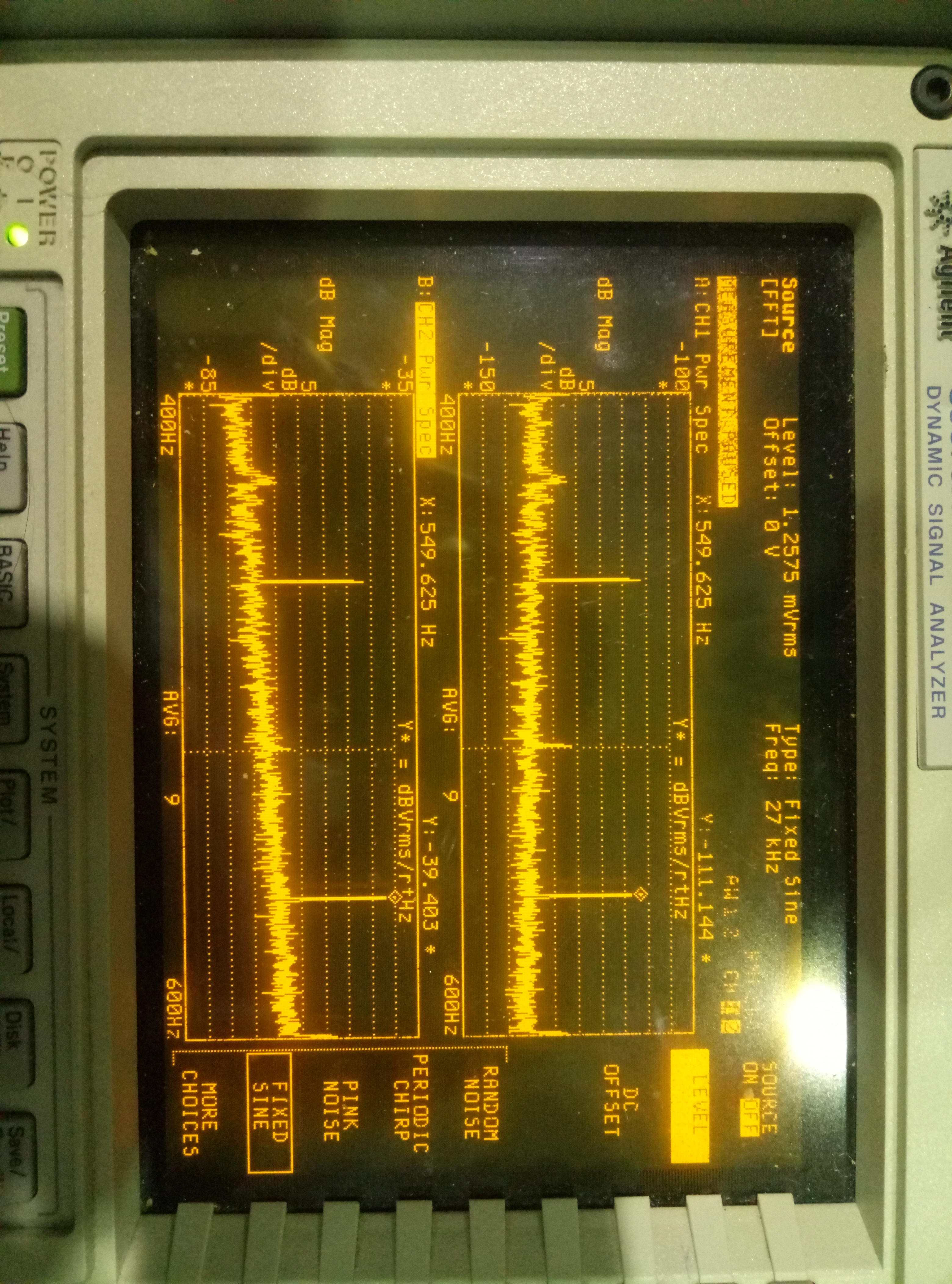
By the way, I also tried to insert noise of 500Hz. It aggres with the prediction, the suspension can filter this high frequency noise. After injecting this noise, we cannot see any peak on the spectrum of PZT or error signal.(See comparation of picture 2 and 3)
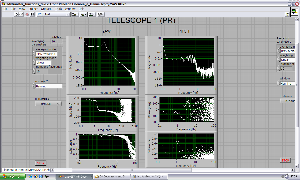
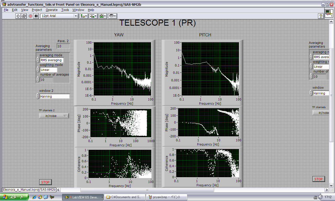
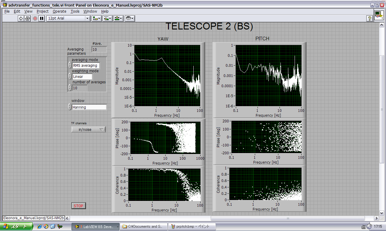
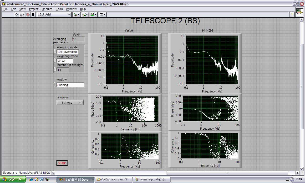
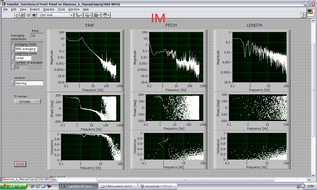
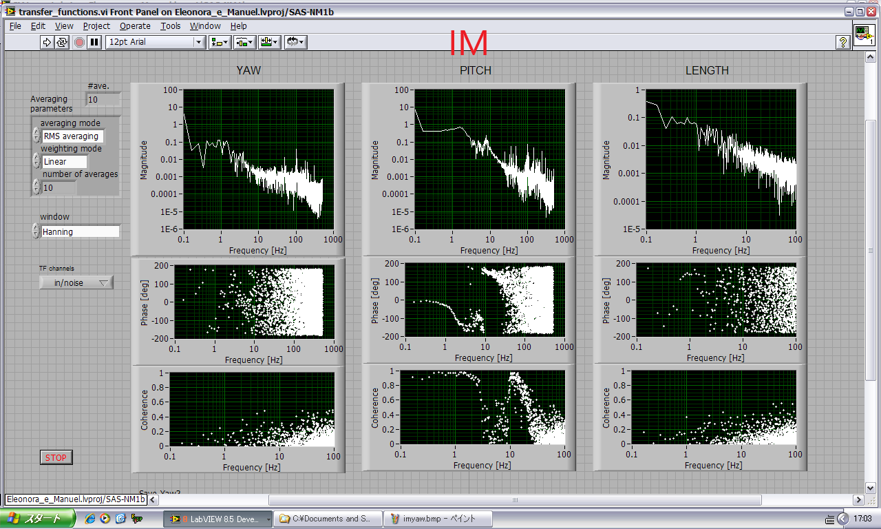
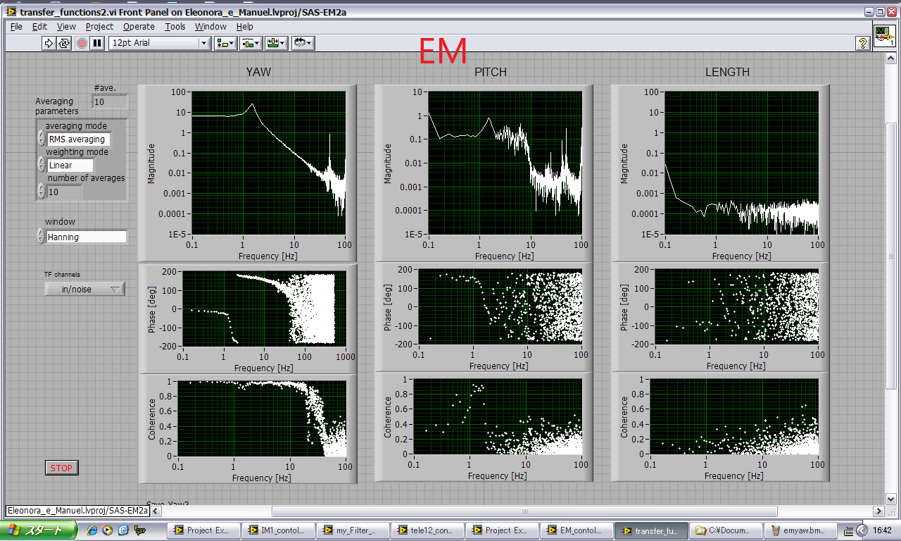
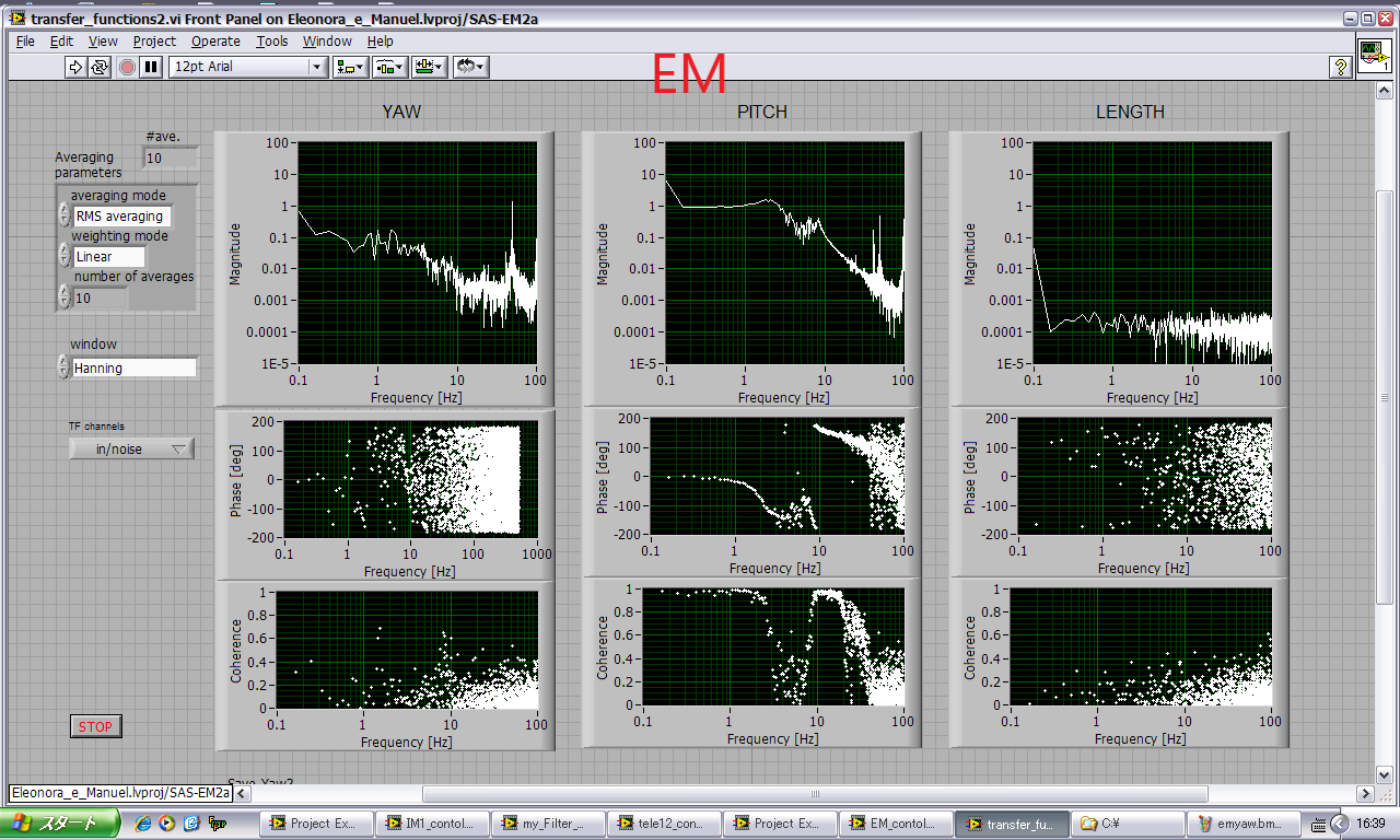
Mechanical transfer functions of local controls as of 21 February 2018.
Noise amplitude: 500mV (white noise injected into port NOISE 2)