- Maps to Science
- Protoplanetary disks/Protostars
- Deriving physical properties of a dust disk from a continuum image
- Understanding rotation of a gas disk from a line cube image
- Star-forming regions
- Using Dendrogram (coming soon)
- Galaxies
- Nearby Galaxy: M100 CO molecular emission line data (coming soon)
- Distant Galaxy: BR1202 [CII] line data (coming soon)
- Active Galactic Nuclei
- (in preparation)
Protoplanetary disks/Protostars
Protoplanetary disks: Understanding rotation of a gas disk from a line cube image
Here are some examples for typical data analyses using the images (maps).Jupyter Notebook version script
We also prepared a Python script in Jupyter Notebook format for the analysis introduced here. You can download the file in Jupyter Notebook format from the following.ipynb file (updated at Feb. 9th, 2024)
Jupyter Notebook needs be installed to run the script. You will also need to install the CASA module into Python (a tarball-installed CASA is not supported). Jupyter Notebook scripts can also be executed on Google Colaboratory (*) (The necessary CASA modules will be installed automatically if the script runs in the Google Colab environment).
Note that the Jupyter Notebook script does not include all the analysis steps described below. For example, each step is realized without using CASA task
viewer.
* Google Colaboratory (abbreviation: Colab) is a service that allows you to write and execute Python from a browser provided by Google. You can read and execute scripts written in Jupyter Notebook format.
The following analysis steps have been confirmed to work with CASA 6.1 (Python 3). The tasks in CASA 5 (Python 2) should work fine, but some Python commands may not work with Python 2.
Getting the image data
The data used this time is the line cube image of H2CO molecule emission for the protoplanetary disk around HL Tau, which was observed with ALMA.In the ALMA Science Archive, please search for:
- Project code: 2018.1.01037.S
- Source Name: HL_Tau
ALMA01424659_00_00_00.fits
can be downloaded directly from
JVO's site
Displaying the FITS image
Please use the taskviewer.
# In CASA
viewer
# In command line
%casaviewer&
viewer.
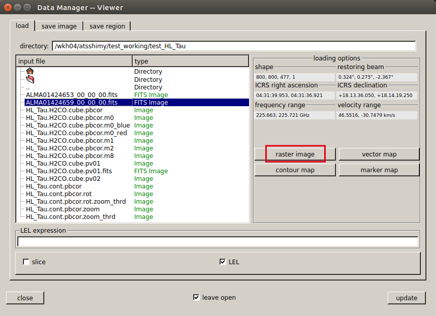 Besides the "Viewer Display Panel", a window called "Data Manager" opens.
Select the data you want to open here and click "raster image".
In addition to image data in CASA format, image FITS files can also be opened directly.
Besides the "Viewer Display Panel", a window called "Data Manager" opens.
Select the data you want to open here and click "raster image".
In addition to image data in CASA format, image FITS files can also be opened directly.
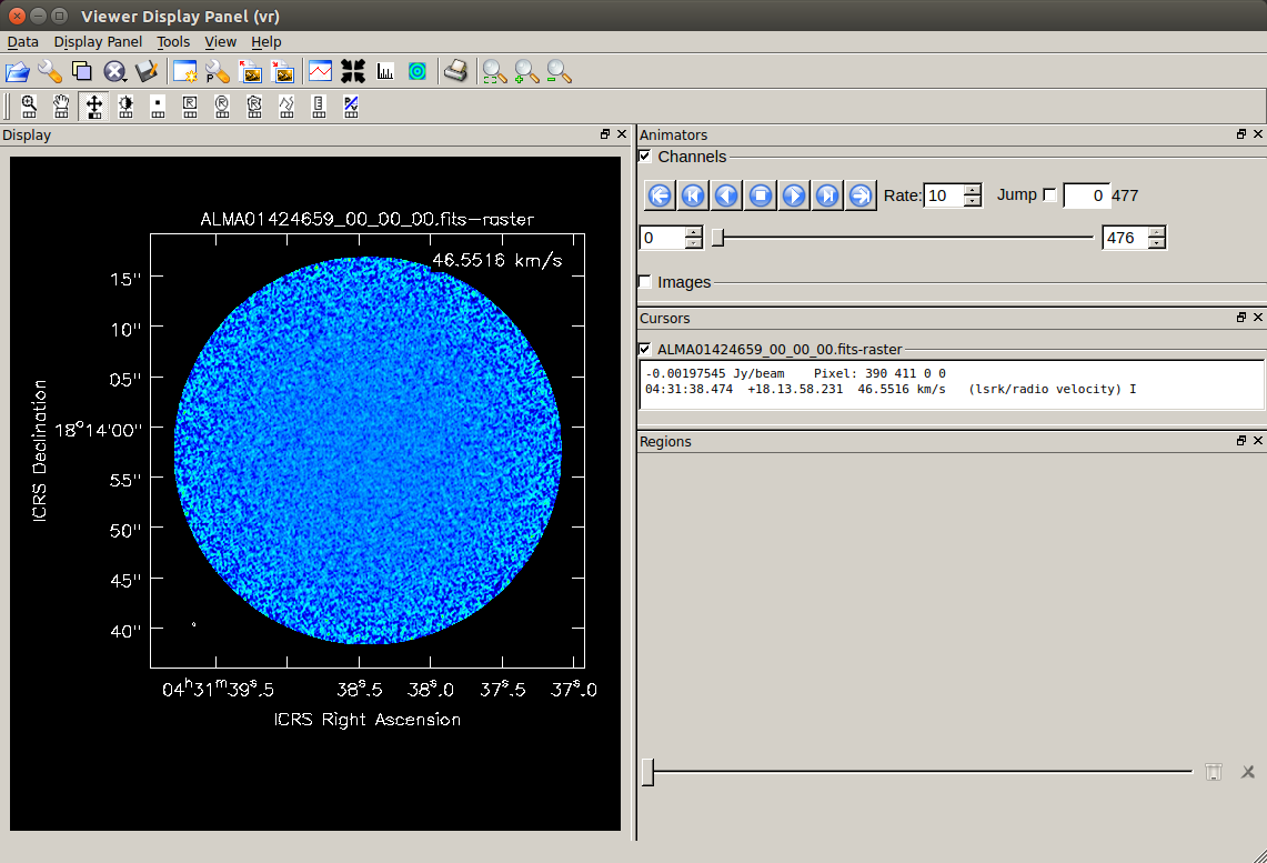 The image of the selected image data is displayed in the "Viewer Display Panel".
 The image file handled here is a cube, so it has information in the frequency (velocity) in the 3rd axis in addition to X and Y.
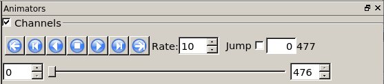
You can disply different channels in frequency using the following buttons.
The image file handled here is a cube, so it has information in the frequency (velocity) in the 3rd axis in addition to X and Y.
You can disply different channels in frequency using the following buttons.

 Channel change (movie)
 Channel shift (by 1ch)
 Stop movie
 Move to min/max channel
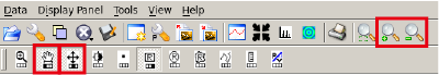 You can perform various operations by clicking each icon on the upper panel of "Viewer Display Panel".
 Zoom in/out
 Move (mouse-drag on screen)
 Change color tone (mouse-drag on screen)
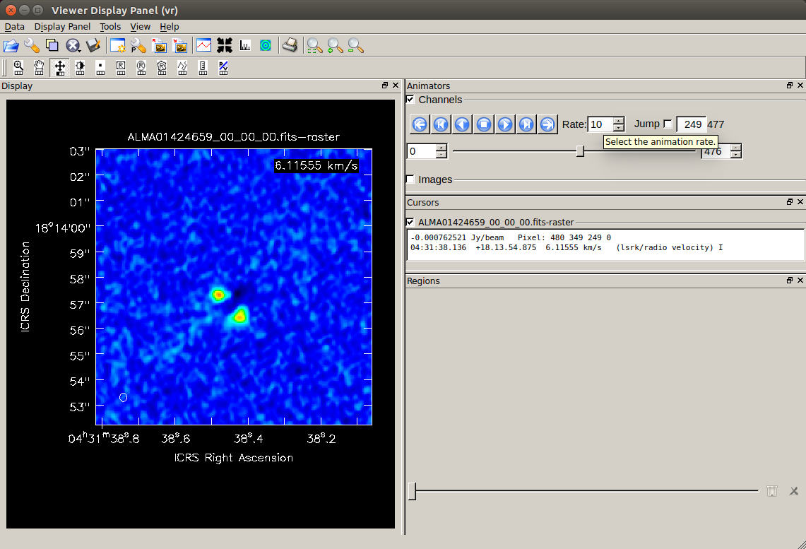 As an example, the right image is the zoom-in, H2CO emission line map of HL Tau with 249 channels (6.11555 km/s).
For information on how to use
viewer, please also refer to the page of "Viewing Images" in CASA docs.
Converting FITS to CASA image format
# In CASA
inimfits='ALMA01424659_00_00_00.fits'
imname = 'HL_Tau.H2CO.cube.pbcor'
importfits(fitsimage=inimfits,
imagename=imname, overwrite=True)
importfits converts the image in FITS to CASA format.
Checking synthesized beam size from the file header
# In CASA
imname = 'HL_Tau.H2CO.cube.pbcor'
imhd_A_res = imhead(imname)
bmaj =imhd_A_res['restoringbeam']['major']['value']
bmajut=imhd_A_res['restoringbeam']['major']['unit']
bmin =imhd_A_res['restoringbeam']['minor']['value']
bminut=imhd_A_res['restoringbeam']['minor']['unit']
bmpa =imhd_A_res['restoringbeam']['positionangle']['value']
bmpaut=imhd_A_res['restoringbeam']['positionangle']['unit']
print('Synthesized Beam:')
print(f' Major Axis = {bmaj:.7f} {bmajut}')
print(f' Minor Axis = {bmin:.7f} {bminut}')
print(f' Pos. Angle = {bmpa:.7f} {bmpaut}')
Synthesized Beam:
Major Axis = 0.3242316 arcsec
Minor Axis = 0.2745839 arcsec
Pos. Angle = -2.3669729 deg
imhead.
This allows you to check not only the beam size but also the coordinate information and frequency information of each axis of the image data.
Displaying a spatially averaged spectrum
You can use the taskviewer to create a spatially-average spectrum from the cube data. After opening the cube with
viewer, please set a region for the spectrum using any of the Mean, Median, Sum, Flux Density and the horizontal axis from channel, radio velocity [km/s], frequency [GHz], etc.
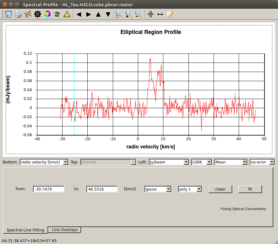 This is the spatially-averaged spectrum within a circle with a radius of 9" from the center of the field of view. It can be seen that a double-peak emission line is detected.
You can check the frequency ranges with and without emission line, and the central velocity of the line (which is expected to be equivalent to the systemic velocity, the velocity of the protostar system itself).
Checking RMS (and emission peak)
# In CASA
imname = 'HL_Tau.H2CO.cube.pbcor'
ctx=400 ; cty=400 # center pixs
stats1=imstat(imagename=imname,
region='circle[['+str(ctx)+'pix,'+str(cty)+'pix],9.0arcsec],range=[30pix,180pix]')
stats2=imstat(imagename=imname,
region='circle[['+str(ctx)+'pix,'+str(cty)+'pix],9.0arcsec],range=[300pix,450pix]')
imgrms=(stats1['rms'][0]+stats2['rms'][0])/2
print(f'RMS [mJy/beam] of {imname} : {imgrms*1000:.7f}')
stats3=imstat(imagename=imname,
region='circle[['+str(ctx)+'pix,'+str(cty)+'pix],4.5arcsec],range=[200pix,280pix]')
imgmax=stats3['max'][0]
print(f'Max [mJy/beam] of {imname} : {imgmax*1000:.7f}')
RMS [mJy/beam] of HL_Tau.H2CO.cube.pbcor : 1.8930310
Max [mJy/beam] of HL_Tau.H2CO.cube.pbcor : 53.1570651
imstat computes statistics such as image RMS and peak values within an area specified by the parameter region. As the "region",
- "circle" specifies a circular area by setting the center position and radius.
- "range" specifies the range (start point, end point) of the frequency/velocity channel.
For more information on how to specify the region, please see the CASA docs "Region File Format".
When measuring the image RMS (noise level), please try to measure in a region without emission from the object. In the above example, the RMS is obtained by specifying the frequency channel where no emission line is detected in "range".
The obtained statistics are read in the form of a Python dictionary object. In addition to RMS, you can also check the maximum and minimum values (and their positions), sum, average of the flux density, etc.
If you want to see all the statistical information, you can print them like the following after running the previous command:
# In CASA
print(stats1)
These statistics can be easily checked on the
viewer, although the way to set a region is different compared to using the CASA task in a command line.
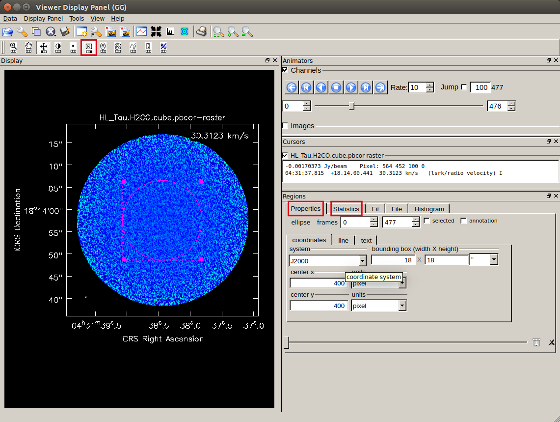 First, please select and display the frequency (velocity) channel that you want to check.
If you want to look at the image RMS, it is a good idea to measure it in the line-free channel.
You can specify a region by clicking on the elliptical region selection button (center of
First, please select and display the frequency (velocity) channel that you want to check.
If you want to look at the image RMS, it is a good idea to measure it in the line-free channel.
You can specify a region by clicking on the elliptical region selection button (center of 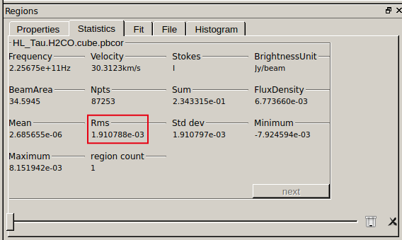 After setting the region, open the "Statistics" tab and you can see statistics including RMS measured in the selected region.
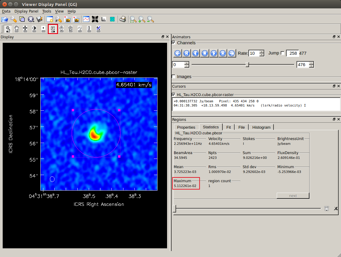 Selecting a region surrounding the line emission from the object will reveal such as the peak flux density as well.
Please note that when obtaining statistics with
viewer, the frequency (velocity) channel used for the statistics is the only one channel which is shown in a display. Also, only rectangular, elliptical (both without rotation), and polygonal are avilable for the shape of a "region".
Making moment maps
The image for line emission is in a form of a 3D image cube with two spatial axes and one frequency (or velocity) axis. These three image planes can be used to create moment maps.# In CASA
imname = 'HL_Tau.H2CO.cube.pbcor'
imname_m0 = imname+'.m0'
imname_m1 = imname+'.m1'
imname_m2 = imname+'.m2'
imname_m8 = imname+'.m8'
imgrms=1.8930310/10**3 #Jy/beam RMS
ctx=402 ; cty=391 ; mwd=180 # center pixs & image size
os.system('rm -rf '+imname+'.m*')
# moment0 & moment8
immoments(imagename = imname, outfile = imname_m0,
axis = 'spectral', moments = 0,
chans = '200~280',
region = 'centerbox[['+str(ctx)+'pix,'+str(cty)+'pix],['+str(mwd)+'pix,'+str(mwd)+'pix]]')
immoments(imagename = imname, outfile = imname_m8,
axis = 'spectral', moments = 8,
chans = '200~280',
region = 'centerbox[['+str(ctx)+'pix,'+str(cty)+'pix],['+str(mwd)+'pix,'+str(mwd)+'pix]]')
# moment1 & moment2
immoments(imagename = imname, outfile = imname_m1,
axis = 'spectral', moments = 1,
chans = '200~280', includepix=[imgrms*5.0, 9999.],
region = 'centerbox[['+str(ctx)+'pix,'+str(cty)+'pix],['+str(mwd)+'pix,'+str(mwd)+'pix]]')
immoments(imagename = imname, outfile = imname_m2,
axis = 'spectral', moments = 2,
chans = '200~280', includepix=[imgrms*5.0, 9999.],
region = 'centerbox[['+str(ctx)+'pix,'+str(cty)+'pix],['+str(mwd)+'pix,'+str(mwd)+'pix]]')
Note that when creating the moment maps here, only the area near the center of the disk (where the center position is (x,y) = (402pix,391pix)) is cut out.
ctx, cty, mwd specify the disk central position and cropped image size in pixels, respectively.
Also, the moment 1 and moment 2 maps are created using only pixels with the flux density at 5σ or above to avoid the significant influence of noise.
Please specify the image RMS measured earlier in imgrms.
 You can check the created moment map with
 viewer. You can open multiple moment maps and display them in animation.
There are other types of moment maps as follows. Each can be created by specifying the following values for the parameter
moments in the task immoments.
- moments=-1 - mean value of the spectrum
- moments=0 - integrated value of the spectrum
- moments=1 - intensity weighted coordinate; traditionally used to get 'velocity fields'
- moments=2 - intensity weighted dispersion of the coordinate; traditionally used to get 'velocity dispersion'
- moments=3 - median of I
- moments=4 - median coordinate
- moments=5 - standard deviation about the mean of the spectrum
- moments=6 - root mean square of the spectrum
- moments=7 - absolute mean deviation of the spectrum
- moments=8 - maximum value of the spectrum
- moments=9 - coordinate of the maximum value of the spectrum
- moments=10 - minimum value of the spectrum
- moments=11 - coordinate of the minimum value of the spectrum
- CASA Docs: "Spectral Analysis"
- CASA Toolkit Reference Manual: "Compute moments from an image"
Comparing with continuum image
You can use theviewer to display the zero moment map (integrated intensity map) with an overlay of the continuum map.
In principle, each image is assumed to be created with the same cell size, image size, and image center (phasecenter).
For the continuum map, we use the CASA format image data (HL_Tau.cont.pbcor) created in "Deriving physical properties of a dust disk from a continuum image".
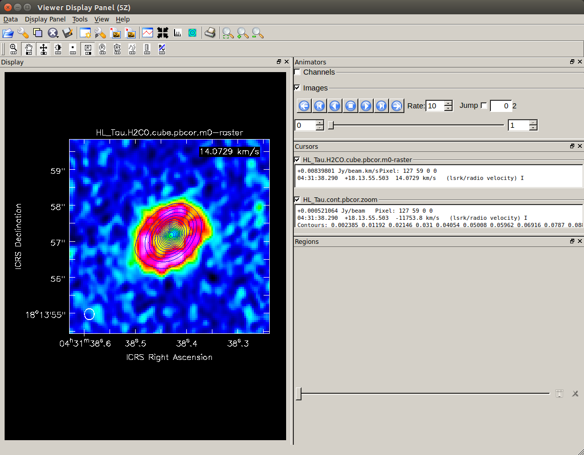 Here is the color image of the moment zero map overlaid with the contours of the continuum map.
From this figure, we can for example see that the positions of the dust disk and the gas disk are roughly the same. Also, it seems that the gas disk is slightly larger here.
Estimating an apparent position angle of the gas disk
If a rough estimate is acceptable, you can use the ruler tool (viewer to obtain the X and Y lengths of the major axis in the moment 0 map you created earlier, so you can estimate the position angle (PA) of the major axis. It is also possible to make a moment 0 map (integrated intensity map) separately for the redshifted component and the blueshifted component, and estimate the PA of the major axis from the shift of their positions.
Moment 0 maps for redshifted and blueshifted components are created as follows.
# In CASA
imname = 'HL_Tau.H2CO.cube.pbcor'
imname_m0a = imname+'.m0_red'
imname_m0b = imname+'.m0_blue'
ctx=402 ; cty=391 ; mwd=180 # center pixs & image size
sysch=243 # channel of system velocity
offch=13 # offset channel for red/blue shift components
os.system('rm -rf '+imname+'.m0_red '+imname+'.m0_blue')
immoments(imagename = imname, outfile = imname_m0a,
axis = 'spectral', moments = 0, chans = '200~'+str(sysch-offch),
region = 'centerbox[['+str(ctx)+'pix,'+str(cty)+'pix],['+str(mwd)+'pix,'+str(mwd)+'pix]]')
immoments(imagename = imname, outfile = imname_m0b,
axis = 'spectral', moments = 0, chans = str(sysch+offch)+'~280',
region = 'centerbox[['+str(ctx)+'pix,'+str(cty)+'pix],['+str(mwd)+'pix,'+str(mwd)+'pix]]')
sysch, the offset before and after the systemic velocity is specified by offch, and the plus side and minus side are used as red and blue shift components to create a moment map.
Here we have sysch=243, offch=13, which means to integrates the 200~230 channels as the redshift component and the 256~280 channels as the blueshift component to create the moment 0 maps.
This will create two maps: HL_Tau.H2CO.cube.pbcor.m0_red, HL_Tau.H2CO.cube.pbcor.m0_blue. Then you can try to measure the center position of the two moment 0 maps of redshift and blueshift using Gaussian fit by
viewer as follows.
- Load an image
- Adjust the display zoom and position of the target source
- Set a region to include the whole area of emission
- Open the "Fit" tab from "Regions" at the bottom right and click "gaussfit"
- Check the position of the fitted Gaussian (Xcen, Ycen)
(x,y) = [97.5716, 97.4801] pixels and the blueshifted peak at (x,y) = [81.3155, 81.0002] pixels.
Therefore, the PA of the major axis can be estimated as follows (# In CASA
import math
incrx = 0.054 # arcsec : pixel interval in X direction (cell size when imaging)
incry = incrx # arcsec : pixel interval in Y direction
cnt_rd = [97.5716, 97.4801] # pixel : peak position of redshift component
cnt_bl = [81.3155, 81.0002] # pixel : Peak position of blue shift component
dxx = cnt_rd[0] - cnt_bl[0] # pixel
dyy = cnt_rd[1] - cnt_bl[1] # pixel
#
gdkpa = 90. + math.degrees(math.atan2( math.sin(math.radians(dxx*incrx)), math.tan(math.radians(dyy*incry)) ))
print(f'Gas disk PA (position angle) = {gdkpa:.5f} deg')
Gas disk PA (position angle) = 134.60488 deg
 Using
Using viewer, you can overlay the moment 0 map for the entire velocity range in color and the moment 0 map for the red- or blue-shifted component in contour.
On both sides in the major-axis direction of the disk, you can see that the upper right is the red-shifted component (on the positive side of the systemic velocity) and the lower left is the blue-shifted component (on the negative side of the systemic velocity). From this, it can be inferred that the disk is rotating around an axis close to the minor axis direction.
Making PV maps
The image cube contains 3D information consisting of two spatial direction XY components and frequency (velocity) component. Normally, when you display a cube data usingviewer etc., you will see a 2D image in X and Y.
On the other hand, the intensity distribution in frequency (velocity) direction and any of the spatial directions is called a position-velocity map (PV map).
The dynamics of a gas disk can be understood from such a PV map created along the major and minor axes with respect to the center of the disk.
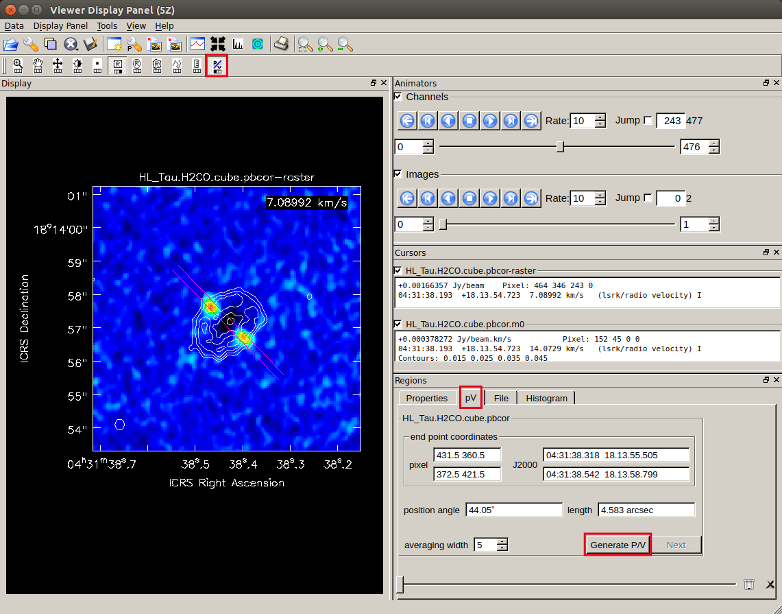
PV maps can be easily created using
viewer as follows. After displaying the cube data, click the "P/V Tool" (
averaging width represents the average width in pixels perpendicular to the slicing direction.
Increasing this value should improve the signal-to-noise ratio of the PV map.
 First, create a PV map along the disk major axis.
In the image on the right, the background is a cube image in color and the moment 0 map is shown with contours.
First, create a PV map along the disk major axis.
In the image on the right, the background is a cube image in color and the moment 0 map is shown with contours. 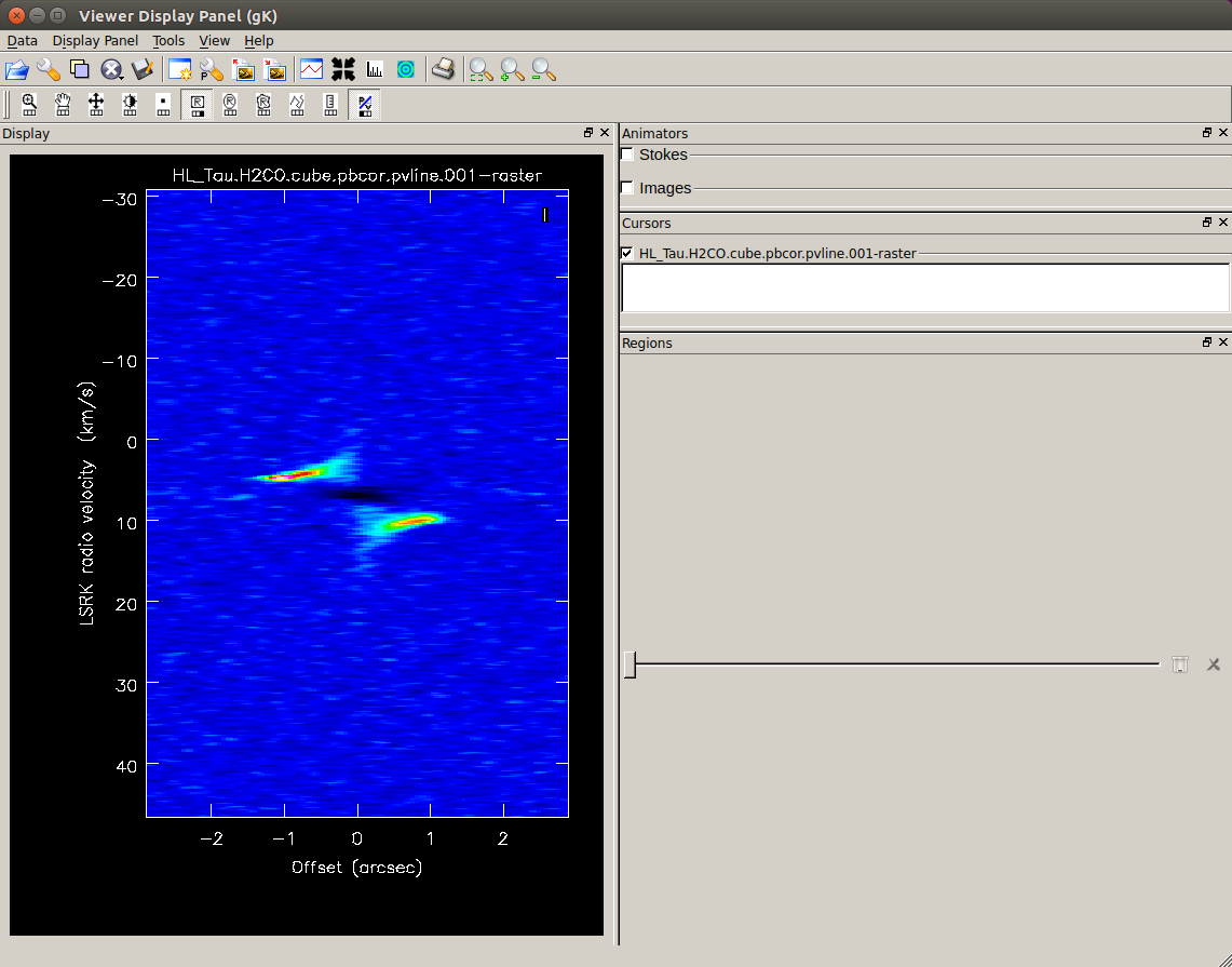 A new window opens, showing the PV map.
Please note that the whole range of the frequency (velocity) in the cube will be used.
A new window opens, showing the PV map.
Please note that the whole range of the frequency (velocity) in the cube will be used.
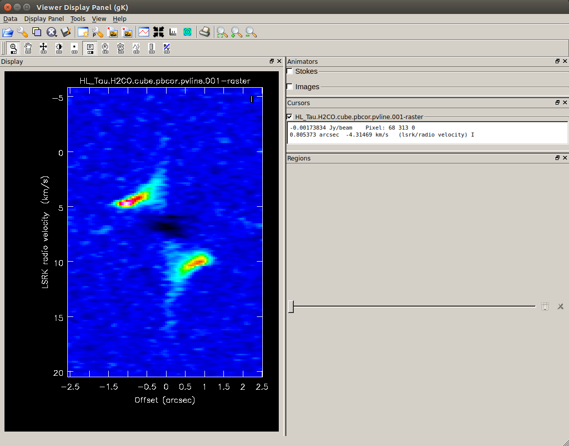 You can always zoom in the image.
The horizontal axis shows the position (offset from the center) and the vertical axis shows the velocity.
You can always zoom in the image.
The horizontal axis shows the position (offset from the center) and the vertical axis shows the velocity.
 When creating a PV map along the disk minor axis,
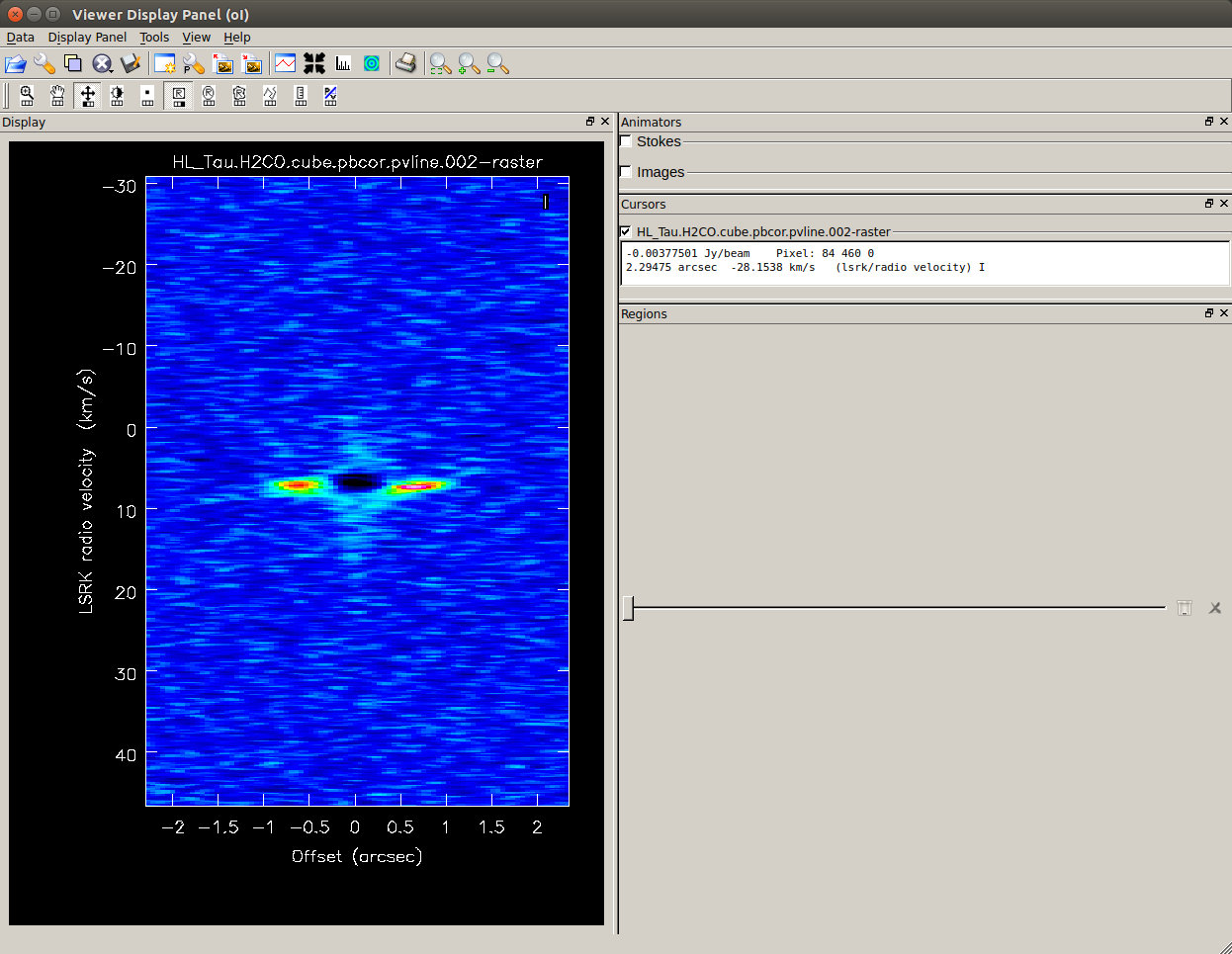 a new window opens, showing the PV map for the minor axis.
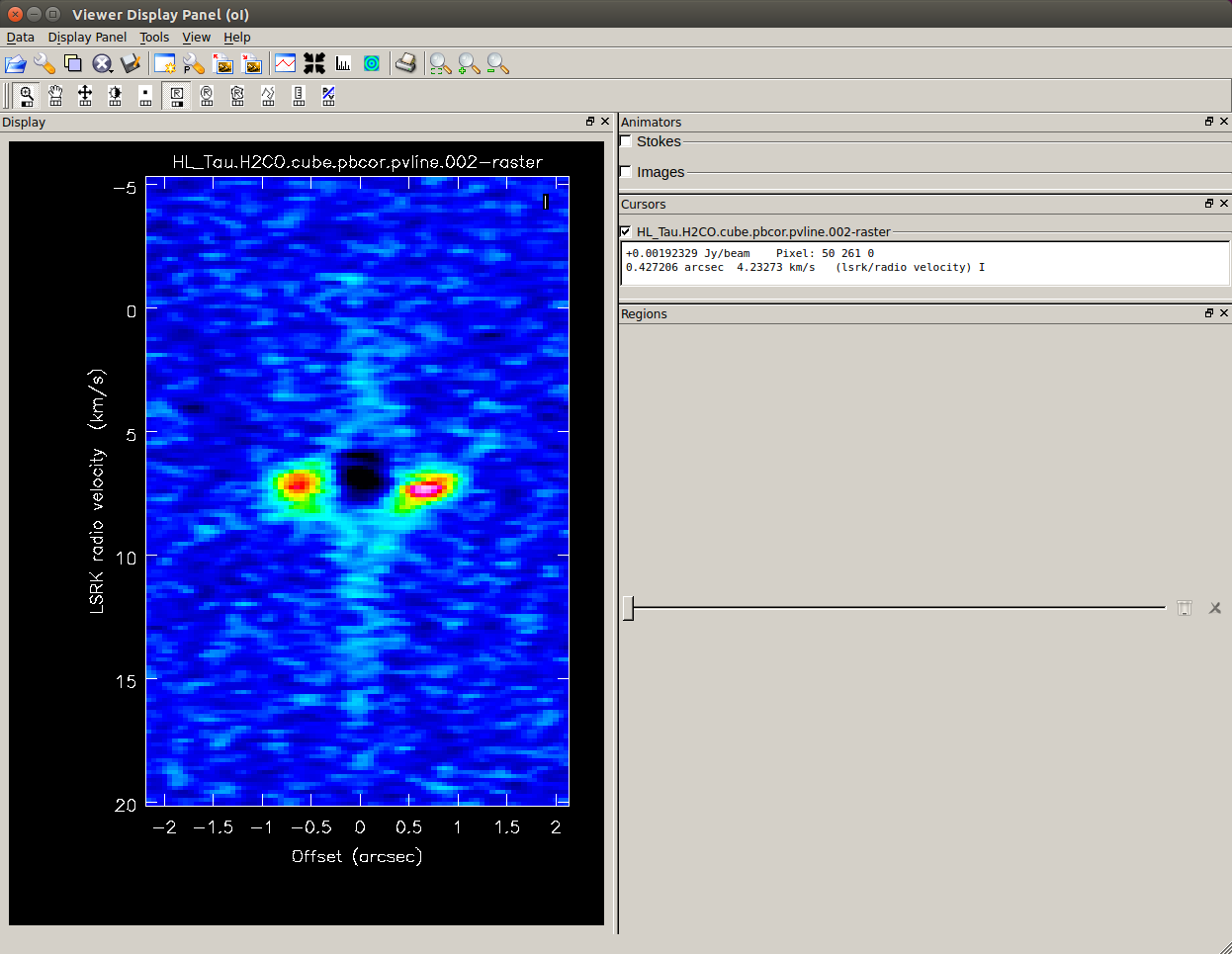 Here is the snap shot after zooming in.
Alternatively, you can also create a PV map using the task
impv as follows: # In CASA
imname = 'HL_Tau.H2CO.cube.pbcor'
pvname1 = 'HL_Tau.H2CO.cube.pv01'
pvname2 = 'HL_Tau.H2CO.cube.pv02'
ctx=402 ; cty=391 # center pixs
pvpa = 134.60 # PA (deg)
plen = 7.0 # arcsec
vlrag = '160~310' # vel.ch.range [ch]
# pv maps
os.system('rm -rf '+pvname1+'*')
impv(imagename = imname, outfile = pvname1,
mode = 'length', center = [ctx, cty],
length = str(pleng)+'arcsec', pa = str(pvpa)+'deg',
width = 5, chans = vlrag)
os.system('rm -rf '+pvname2+'*')
impv(imagename = imname, outfile = pvname2,
mode = 'length', center = [ctx, cty],
length = str(pleng)+'arcsec', pa = str(pvpa+90.)+'deg',
width = 5, chans = vlrag)
# fits
exportfits(imagename=pvname1, fitsimage=pvname1+'.fits',
velocity=True, dropstokes=True, overwrite=True)
impv creates a PV map of length pleng (arcsec) by slicing in the direction of the position angle (PA) pvpa(deg) of the major axis of the disk, and in the direction perpendicular to it (minor axis), based on the center position ctx, cty(pixels).
In the direction of velocity, it is limited to vlrag(channels).
This will lead to two PV maps: HL_Tau.H2CO.cube.pv01, HL_Tau.H2CO.cube.pv02.
Assuming Keplerian rotation, the expected gas rotation curve can be calculated and displayed on the PV diagram (PV map for the major axis). Considering a geometrically thin, axisymmetric gas disk with Keplerian rotation, the rotational velocity at a radius
r from the center is expressed as incl, the line-of-sight component of the rotation speed Vrot is 1.3 Mo, systemic velocity of Vsys = 7.2 km/s, and inclination of the gas disk of incl = 42.5 deg.
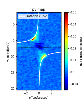 The flux distribution on the PV diagram appears to be in good agreement with the position-velocity profile of the Kepler rotation predicted here.
Note that the dotted black lines in the figure indicate the systemic velocity
The flux distribution on the PV diagram appears to be in good agreement with the position-velocity profile of the Kepler rotation predicted here.
Note that the dotted black lines in the figure indicate the systemic velocity Vsys and the central position (with an offset of zero).
The following is the example script that creates the above image. This script uses Python matplotlib (plotting) and astropy (reading a FITS file) modules to overlay the calculated, expected rotation curve onto the PV map. After creating the PV map in FITS (
HL_Tau.H2CO.cube.pv02.fits) in the previous step, please execute it in the Python environment with matplotlib and astropy installed.
# In Python
import math
from matplotlib import pyplot as plt
from astropy.io import fits
au = 1.49597870700*10**(11) #m/AU
pc = 3.085677581*10**(16) #m/pc
Msol= 1.98847*10**(33) #g Solar mass
Grv = 6.67430*10**(-14) # m3/g s2 Newtonian Constant of Gravitation

# for HL Tau
dist = 140.#pc
stmass = 1.3#Mo
Vsys = 7.2#km/s
incl = 42.5 #deg

pvname1 = 'HL_Tau.H2CO.cube.pv01'
ftdat = fits.open(pvname1+'.fits')
ft_img = ftdat[0].data
ft_hdr = ftdat[0].header
ftdat.close()

NN = int(ft_hdr['NAXIS1']/2.)
dt_rx1 = [[] for _ in range(NN)] ; dt_rx2 = [[] for _ in range(NN)]
dt_vt1 = [[] for _ in range(NN)] ; dt_vt2 = [[] for _ in range(NN)]
for rrr in list(range(NN)):
rrr += 1
radu = dist*pc*math.tan(math.radians(rrr*ft_hdr['CDELT1']/3600))/2 # m
dt_rx1[rrr-1] = -rrr*ft_hdr['CDELT1'] # arcsec
dt_rx2[rrr-1] = rrr*ft_hdr['CDELT1']
dt_vt1[rrr-1] = Vsys - math.sqrt(Grv*(stmass*Msol)/radu)/1000 * math.cos(math.radians(90.-incl)) # km/s
dt_vt2[rrr-1] = Vsys + math.sqrt(Grv*(stmass*Msol)/radu)/1000 * math.cos(math.radians(90.-incl))

ofs_st=(ft_hdr['CRVAL1']+( 1 -ft_hdr['CRPIX1'])*ft_hdr['CDELT1'])
ofs_ed=(ft_hdr['CRVAL1']+(ft_hdr['NAXIS1']-ft_hdr['CRPIX1'])*ft_hdr['CDELT1'])
vel_st=(ft_hdr['CRVAL2']+( 1 -ft_hdr['CRPIX2'])*ft_hdr['CDELT2'])/1000
vel_ed=(ft_hdr['CRVAL2']+(ft_hdr['NAXIS2']-ft_hdr['CRPIX2'])*ft_hdr['CDELT2'])/1000

ff, aa = plt.subplots(1,1, figsize=(4,5))
img = aa.imshow(ft_img, origin='lower', extent=(ofs_st,ofs_ed,vel_st,vel_ed),
vmin=-0.015, vmax=0.05, cmap='jet')
aa.set_xlabel("offset[arcsec]") ; aa.set_xlim(ofs_st,ofs_ed)
aa.set_ylabel("velocity[km/s]") ; aa.set_ylim(vel_st,vel_ed)
aa.set_aspect(0.5)
cbar=plt.colorbar(img, ax=aa)
cbar.set_label("flux density ["+ft_hdr['BUNIT']+"]",size=9)
aa. set_title('pv map')
plt.vlines( [0], vel_st, vel_ed, "black", linewidth = 0.7, linestyles='dashed')
plt.hlines([Vsys], ofs_st, ofs_ed, "black", linewidth = 0.7, linestyles='dashed')
imr = aa.plot(dt_rx1, dt_vt1, "-", color='white', linewidth = 2.0, label="rotation curve")
imr = aa.plot(dt_rx2, dt_vt2, "-", color='white', linewidth = 2.0)
aa.legend(loc="upper left")
plt.savefig('line_pvmap_model.png')
back to top
Last Update: 2024.02.15