- Maps to Science
- Protoplanetary disks/Protostars
- Deriving physical properties of a dust disk from a continuum image
- Understanding rotation of a gas disk from a line cube image
- Star-forming regions
- Using Dendrogram (coming soon)
- Galaxies
- Nearby Galaxy: M100 CO molecular emission line data (coming soon)
- Distant Galaxy: BR1202 [CII] line data (coming soon)
- Active Galactic Nuclei
- (in preparation)
Protoplanetary disks/Protostars
Protoplanetary disks: Deriving physical properties of a dust disk from a continuum image
Here are some examples for typical data analyses using the images (maps).Jupyter Notebook version script
We also prepared a Python script in Jupyter Notebook format for the analysis introduced here. You can download the file in Jupyter Notebook format from the following.ipynb file (updated at Feb. 9th, 2024)
Jupyter Notebook needs be installed to run the script. You will also need to install the CASA module into Python (a tarball-installed CASA is not supported). Jupyter Notebook scripts can also be executed on Google Colaboratory (*) (The necessary CASA modules will be installed automatically if the script runs in the Google Colab environment).
Note that the Jupyter Notebook script does not include all the analysis steps described below. For example, each step is realized without using CASA task
viewer.
* Google Colaboratory (abbreviation: Colab) is a service that allows you to write and execute Python from a browser provided by Google. You can read and execute scripts written in Jupyter Notebook format.
The following analysis steps have been confirmed to work with CASA 6.1 (Python 3). The tasks in CASA 5 (Python 2) should work fine, but some Python commands may not work with Python 2.
Getting the image data
The image used this time is the continuum image of the protoplanetary disk around HL Tau, which was observed with ALMA.In the ALMA Science Archive, please search for:
- Project code: 2018.1.01037.S
- Source Name: HL_Tau
ALMA01424653_00_00_00.fits
can be downloaded directly from JVO's site. Displaying the FITS image
Please use the taskviewer.
# In CASA
viewer
# In command line
%casaviewer&
viewer.
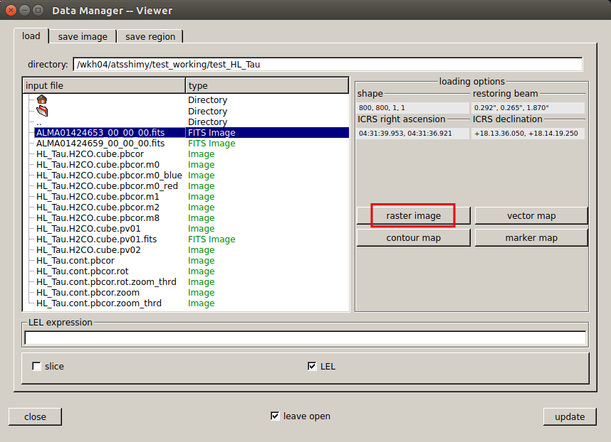 Besides the "Viewer Display Panel", a window called "Data Manager" opens.
Select the data you want to open here and click "raster image".
In addition to image data in CASA format, image FITS files can also be opened directly.
Besides the "Viewer Display Panel", a window called "Data Manager" opens.
Select the data you want to open here and click "raster image".
In addition to image data in CASA format, image FITS files can also be opened directly.
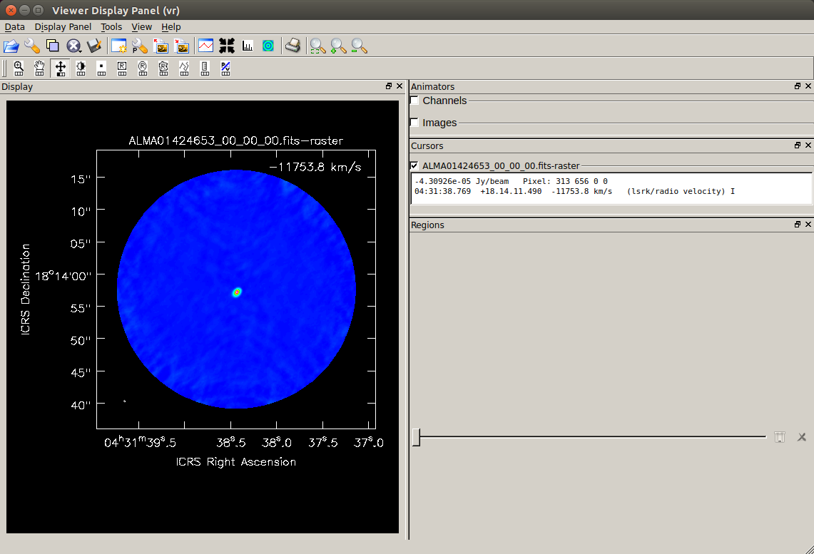 The image of the selected image data is displayed in the "Viewer Display Panel".
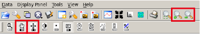 You can perform various operations by clicking each icon on the upper part of "Viewer Display Panel".
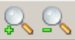 Zoom in/out
 Move (mouse-drag on screen)
 Change color tone (mouse-drag on screen)
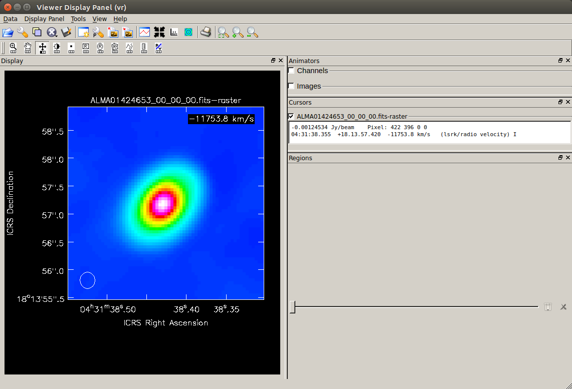 For example, this is an zoomed-in continuum image of HL Tau.
For information on how to use
viewer, please also refer to the page of "Viewing Images" in CASA docs.
Converting FITS to CASA image format
# In CASA
inimfits='ALMA01424653_00_00_00.fits'
imname = 'HL_Tau.cont.pbcor'
importfits(fitsimage=inimfits,
imagename=imname, overwrite=True)
importfits converts the image in FITS to CASA format.
Please specify the input image FITS name for fitsimage, and the output CASA format file name (actually a directory) for imagename.
Checking synthesized beam size (and frequency) from the file header
# In CASA
imname = 'HL_Tau.cont.pbcor'
imhd_A_res = imhead(imname)
bmaj =imhd_A_res['restoringbeam']['major']['value']
bmajut=imhd_A_res['restoringbeam']['major']['unit']
bmin =imhd_A_res['restoringbeam']['minor']['value']
bminut=imhd_A_res['restoringbeam']['minor']['unit']
bmpa =imhd_A_res['restoringbeam']['positionangle']['value']
bmpaut=imhd_A_res['restoringbeam']['positionangle']['unit']
print('Synthesized Beam:')
print(f' Major Axis = {bmaj:.7f} {bmajut}')
print(f' Minor Axis = {bmin:.7f} {bminut}')
print(f' Pos. Angle = {bmpa:.7f} {bmpaut}')
cfreq =imhd_A_res['refval'][2]
frequt=imhd_A_res['axisunits'][2]
if frequency == 'Hz':
cfreqgh = cfreq/10**(9)
print(f'Observing Frequency = {cfreqgh:.6f} GHz')
else:
print(f'Observing Frequency = {cfreq:.1f} {frequt}')
Synthesized Beam:
Major Axis = 0.2922270 arcsec
Minor Axis = 0.2649764 arcsec
Pos. Angle = 1.8701019 deg
Observing Frequency = 235.541305 GHz
imhead.
This allows you to check not only the beam size but also each coordinate/frequency axis value, pixel scale, number of pixels, etc. of the image data.
In addition, the observation frequency is also confirmed in the above example.
Checking RMS and peak values in the image
# In CASA
imname = 'HL_Tau.cont.pbcor'
stats1=imstat(imagename=imname, region='box[[260pix,265pix],[360pix,535pix]]')
stats2=imstat(imagename=imname, region='box[[440pix,265pix],[540pix,535pix]]')
imgrms=(stats1['rms'][0]+stats2['rms'][0])/2
print(f'RMS [mJy/beam] of {imname} : {imgrms*1000:.7f}')
RMS [mJy/beam] of HL_Tau.cont.pbcor : 0.4689696
# In CASA
imname = 'HL_Tau.cont.pbcor'
ctx=400 ; cty=400 # center pixs
stats1=imstat(imagename=imname,
region='annulus[['+str(ctx)+'pix,'+str(cty)+'pix],[4.5arcsec,14.0arcsec]]')
imgrms=stats1['rms'][0]
print(f'RMS [mJy/beam] of {imname} : {imgrms*1000:.7f}')
stats2=imstat(imagename=imname,
region='circle[['+str(ctx)+'pix,'+str(cty)+'pix],4.5arcsec]')
imgmax=stats2['max'][0]
print(f'Max [mJy/beam] of {imname} : {imgmax*1000:.7f}')
RMS [mJy/beam] of HL_Tau.cont.pbcor : 0.4748368
Max [mJy/beam] of HL_Tau.cont.pbcor : 136.6068870
imstat computes statistics such as image RMS and peak values within the range specified by the parameter region. 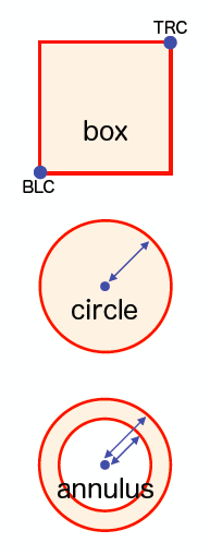 Here is a list of the shape that is frequently used as a "region":
- "box" specifies a rectangular area by setting BLC (bottom left corner) and TRC (top right corner).
- "circle" specifies a circular area by setting the center position and radius.
- "annulus" can specify a ring-shaped area, and set the center position, inner and outer radii of the ring. This is useful for obtaining RMS etc. while avoiding detected objects.
For more information on how to specify the region, see the CASA docs "Region File Format".
When measuring the image RMS (noise level), please try to measure in a region without emission from any (possible) real objects. In the above example, "box" specifies a rectangular area offset from the object, and "annulus" specifies a ring area surrounding the target source.
The obtained statistics are read in the form of a Python dictionary object. In addition to RMS, you can also know the maximum and minimum values (and their positions), sum, average of the flux density, etc.
If you want to see all the statistical information, you can print them like the following after running the previous command:
# In CASA
print(stats1)
These statistics can be easily checked on the
viewer although the way to set a region is different compared to using the CASA task in a command line.
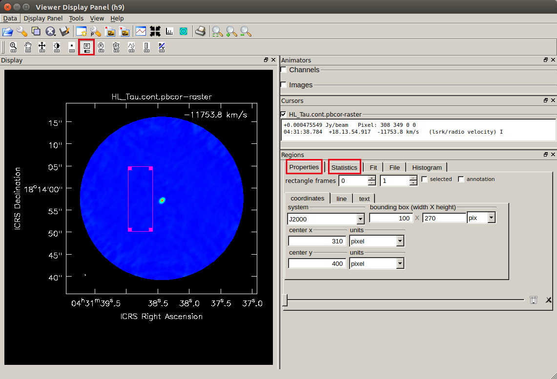 Please click the rectangular region selection button (the left one in
 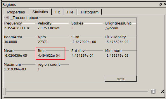 After specifying the region, open the "Statistics" tab and you can see statistics including RMS measured in the selected region.
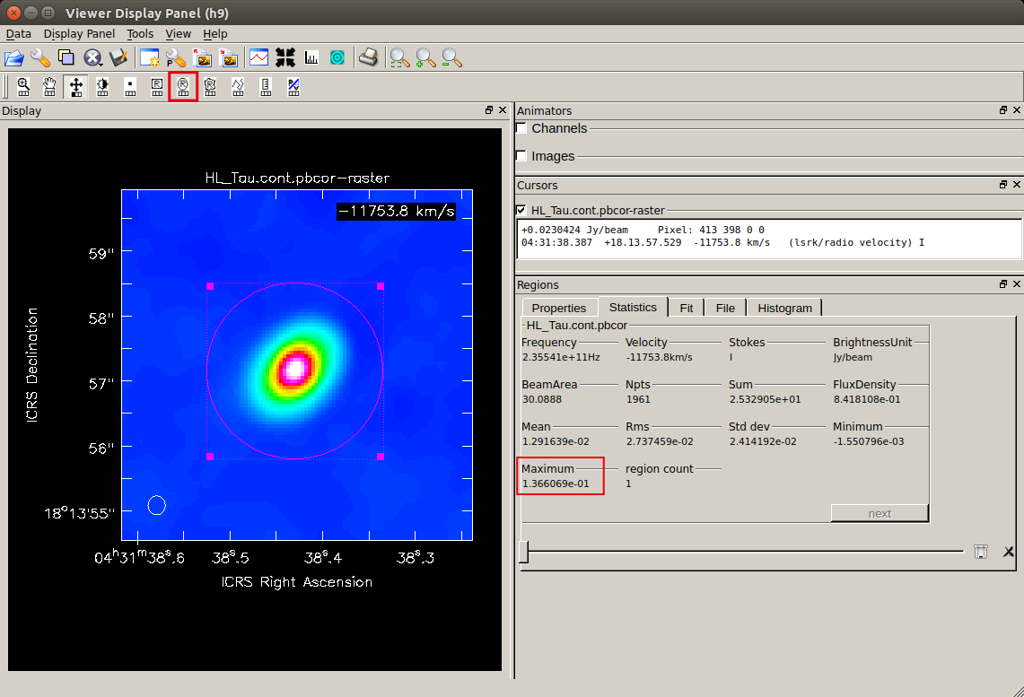 Selecting a region including the continuum emission will reveal such as the peak flux density of this object.
Please note that when obtaining statistics with
viewer, the frequency (velocity) channel used for the statistics is the only one channel which is shown in a display (you do not have to be worried about this since there is only one channel for the continuum map). Also, only rectangular, elliptical (both without rotation), and polygonal are avilable for the shape of a "region".
Estimating a position for a protostar with 2D Gaussian fit
First, here is the steps for the Gaussian fitting inviewer.
- Load image with
viewer - Adjust the image zoom level and position so that the target source can be easily seen
- Specify a region that surrounds the target source
- Open the "Fit" tab from "Regions" at the bottom right and click "gaussfit"
- Ra_ICRS, Dec_ICRS : Center position (absolute coordinates)
- Xcen, Ycen : Center position (pixel)
- W-Majorax, W-Minorax : FWHM of major axis and minor axis (arcsec etc.)
- I-Majorax, I-Minorax : FWHM (pixel) of major axis and minor axis
- IntegrFlux : Total Flux (Jy)
- PeakFlux : Peak flux density (Jy/beam)
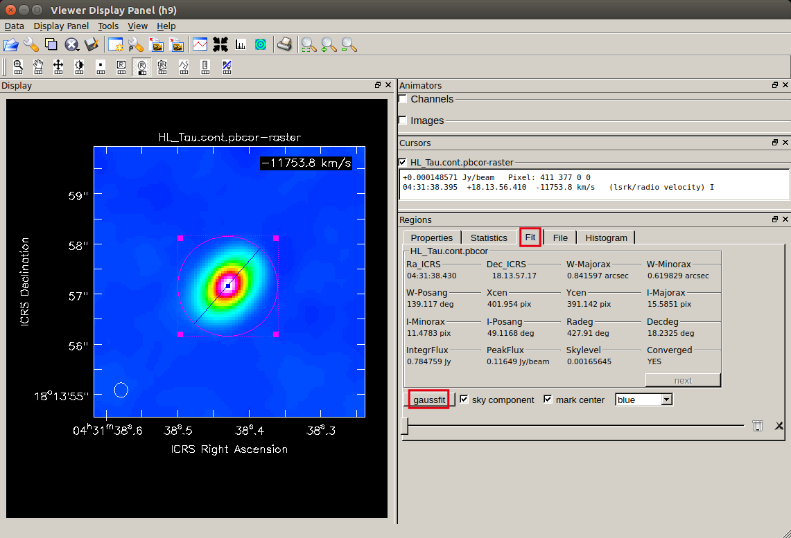 Also, the center position and the direction of the major axis are represented by a straight line on the image.
The position of the protostar can be estimated from the center position of the fitted Gaussian. Please compare the result with the coordinates of the protostar (HL Tau) in any astronomical catalog.
If you do the above from the command line of CASA, it will be as follows. Please use
viewer to roughly check the pixel value of the center position of the target source in advance, and specify the initial values for fitting with ctpix, ctpiy. # In CASA
import math
imname = 'HL_Tau.cont.pbcor'
ctpix = 402 # pix
ctpiy = 391 # pix
xfit_B_res = imfit(imname,
region = 'circle[['+str(ctpix)+'pix,'+str(ctpiy)+'pix],1.5arcsec]',
newestimates = imname+'.imfit_estimates',
logfile = imname+'.imfit_log')
xfit_B=xfit_B_res['results']['component0']
Flux =xfit_B['peak']['value'] ; FluxUn=xfit_B['peak']['unit']
Gmajor=xfit_B['shape']['majoraxis']['value'] ; GmajUn=xfit_B['shape']['majoraxis']['unit']
Gminor=xfit_B['shape']['minoraxis']['value'] ; GminUn=xfit_B['shape']['minoraxis']['unit']
Gpa =xfit_B['shape']['positionangle']['value'] ; GpaUn =xfit_B['shape']['positionangle']['unit']
xxx1 = math.degrees(xfit_B['shape']['direction']['m0']['value'])
yyy1 = math.degrees(xfit_B['shape']['direction']['m1']['value'])
print('Gaussian fit:')
print(" Peak flux = %6.4f %s, FWHM = %6.4f %sx %6.4f %s (PA = %6.4f %s)"
% (Flux,FluxUn,Gmajor,GmajUn,Gminor,GminUn,Gpa,GpaUn))
Gaussian fit:
Peak flux = 0.1164 Jy/beam, FWHM = 0.8656 arcsec x 0.6385 arcsec (PA = 138.9841 deg)
imfit is used for fitting.
From the results of the two-dimensional Gaussian fit, the peak flux density, major and minor axis full width at half maximum (FWHM), and position angle (PA) of the elliptical Gaussian are obtained.
The fitting result is read as a Python dictionary object, and you can check many parameters in addition to the above.
Getting a flux density profile along the major axis
Based on the center position and the position angle PA obtained by the Gaussian fitting, let's create a flux density profile along the disk major axis.You can easily inspect it in
viewer. 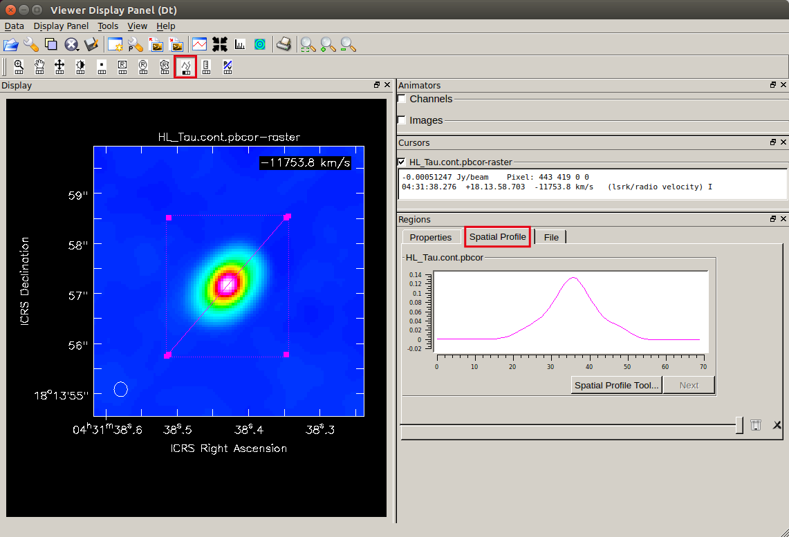
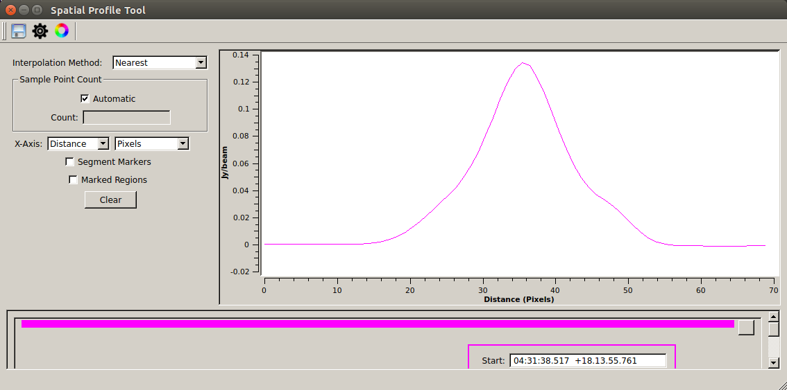
The procedure is as follows:
- Load an image
- Adjust the display zoom and position of the target source
- Specify the line to slice (after selecting
 , click the start point and double click the end point on the screen)
 - Open the "Spatial Profile" tab from "Regions" on the bottom right, then you can see the flux density distribution along the specified straight line
Also, the flux density profile can be extracted to a text file using the CASA Toolkit. If you want to specify the position for the profile strictly, please try this as well.
Referring to the result obtained by the two-dimensional Gaussian fit described above, please specify the pixel value of the center position of the target source with
pixx1, piyy1, specify the position angle PA in the slicing direction for Gpa (it may be the same as the PA of the disk), and specify the slicing length in pixels for hspp.
It will be written to a csv (text) file called cont_majaxis_profile.csv. You can make a plot for the flux density profile using any plotting tools.
# In CASA
import math
import numpy as np
imname = 'HL_Tau.cont.pbcor'
pix1= 402 # pix
piyy1=391# pix
Gpa = 138.98 # PA (deg)
hspp=60 # pix
blcx=int(np.round(pixx1-hspp/2.*math.cos(math.radians(Gpa-90.))))
blcy=int(np.round(piyy1-hspp/2.*math.sin(math.radians(Gpa-90.))))
trcx=int(np.round(pixx1+hspp/2.*math.cos(math.radians(Gpa-90.))))
trcy=int(np.round(piyy1+hspp/2.*math.sin(math.radians(Gpa-90.))))

ia.open(infile=imname)
rec = ia.getslice(x=[blcx,trcx], y=[blcy,trcy], npts=hspp)
ia.close()

path_w = 'cont_majaxis_profile.csv'
rec_dp = [str(n)+','+str(m) for n,m in zip(rec['distance'],rec['pixel'])]
with open(path_w, mode='w') as f:
f.write('\n'.join(rec_dp))
f.close()
Estimating the radius and inclination of a dust disk above 5σ
Considering the apparent area of the continuum image that contains emission above the 5σ level, we obtain the radius and inclination of the dust disk from the major and minor axis diameters.Here is how to measure the spatial scale with
viewer. First, please display the 5σ area with contours in
viewer.
After displaying the continuum image with "raster image", please open the same image with "contour map".
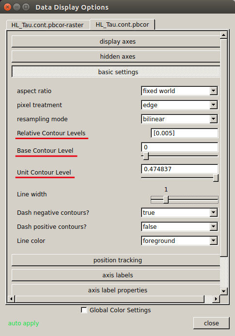 Then please open "Data Display Options" (
- Relative Contour Level=[0.005]
- Base Contour Level=0
- Unit Contour Level=RMS(mJy/beam)
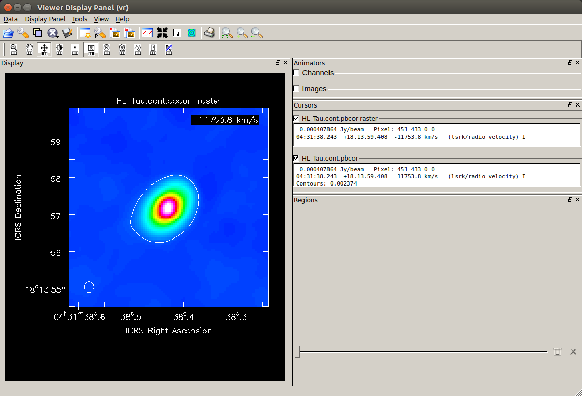 Overlaid on the color image, you can see the line drawn at the 5σ level.
Based on this image, measure the major and minor axis diameters of the area of 5σ or above.
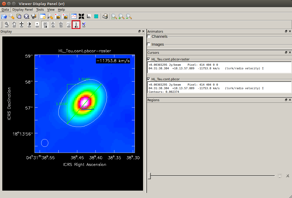 After clicking the ruler tool (
 This is the minor axis, 1.5155".
Based on the major and minor axis sizes obtained above, the radius and inclination of the dust disk are estimated as follows.
# In CASA
import math
majax = 2.0106 # arcsec
minax = 1.5155 # arcsec

au = 1.49597870700*10**(11) #m/AU
pc = 3.085677581*10**(16) #m/pc
dist= 140.# pc @ HL Tau
radi=dist*(pc/au)*math.tan(math.radians(majax/3600))/2
incl=math.degrees(math.asin(minax/majax))
print(f'Disk radius & inclination = {radi:.4f} AU, {incl:.4f} deg')
Disk radius & inclination = 140.7420 AU, 48.9167 deg
i is related to the axial ratio as r of the radius can be calculated assuming the relation, Θ and the distance to the target souce is D.
The distance to HL Tau can be assumed to be 140 [pc].
If you do the above from the command line of CASA, it will be as follows.
# In CASA
import math
import numpy as np
Gpa = 138.98 # PA (deg)
imgrms = 0.4748368 # RMS (mJy/beam)

imname = 'HL_Tau.cont.pbcor'
imname0 = imname + '.rot'
rotpa = -Gpa + 90.
ia.open(infile=imname)
imr = ia.rotate(outfile=imname0, pa=str(rotpa)+GpaUn, overwrite=True)
imr.done()
ia.close()

imname1 = imname0 + '.zoom_thrd'
nsigma = 5.0 #  σ threshold
threshold = (imgrms/1000)*nsigma
ctx=400 ; cty=400 ; iwd=60 # center pixs & image width
blcx=int(ctx-iwd/2) ; trcx=int(ctx+iwd/2)
blcy=int(cty-iwd/2) ; trcy=int(cty+iwd/2)
box1=','.join([str(blcx), str(blcy), str(trcx), str(trcy)])
os.system('rm -rf '+imname1)
immath(imagename=[imname0],
expr='IM0[IM0>%f]'%threshold,
box = box1,
outfile=imname1)

box2=','.join([str(0), str(0), str(iwd-1), str(iwd-1)])
imv_res = imval(imagename=imname1, box=box2)
imv_data = imv_res['data']
imv_mask = imv_res['mask']
imv_dt_tp = imv_data.transpose(1,0)
imv_mk_tp = imv_mask.transpose(1,0)
np.putmask(imv_dt_tp, imv_mk_tp==False, "0")
xslice = imv_dt_tp.sum(0)
yslice = imv_dt_tp.sum(1)
nxpix = np.sum( np.where(xslice > 0, 1, xslice) )
nypix = np.sum( np.where(yslice > 0, 1, yslice) )

imhd_A_res = imhead(imname1)
incrx = abs(math.degrees(imhd_A_res['incr'][0])*3600)
incry = abs(math.degrees(imhd_A_res['incr'][1])*3600)
if nypix*incry >= nxpix*incrx:
Gmajor = nypix*incry
Gminor = nxpix*incrx
else:
Gmajor = nxpix * incrx
Gminor = nypix*incry
print(f'major/minor axes of 5 sigma area = {Gmajor:.4f} [arcsec] x {Gminor:.4f} [arcsec]')

au = 1.49597870700*10**(11) #m/AU
pc = 3.085677581*10**(16) #m/pc
dist= 140.# pc @ HL Tau
radi=dist*(pc/au)*math.tan(math.radians(Gmajor/3600))/2
incl=math.degrees(math.asin(Gminor/Gmajor))
print(f'Disk radius & inclination = {radi:.4f} AU, {incl:.4f} deg')
Estimating dust mass from the total flux above 5σ
You can use the taskimmath as following to create an image that cuts out the regions above the 5σ level threshold.
In addition, the task imstat can calculate the total flux from the continuum map above 5σ. imgrms means the image RMS. Please use the value you found earlier for RMS. In the following example, the central part of the disk is extracted with the 5σ level threshold.
If you want to change the threshold from 5σ, please change nsigma. # In CASA
imname = 'HL_Tau.cont.pbcor'
imname2 = imname+'.zoom_thrd'
imgrms = 0.4748368 # RMS (mJy/beam)
nsigma = 5.0 # <nsigma> σ threshold
threshold = (imgrms/1000)*nsigma
ctx=402 ; cty=391 ; iwd=60 # center pixs & image width
blcx=int(ctx-iwd/2) ; trcx=int(ctx+iwd/2)
blcy=int(cty-iwd/2) ; trcy=int(cty+iwd/2)
box3=','.join([str(blcx), str(blcy), str(trcx), str(trcy)])
os.system('rm -rf '+imname2)
immath(imagename=[imname],
expr='IM0[IM0>%f]'%threshold,
box = box3,
outfile=imname2)
stats=imstat(imagename=imname2)
imgflx=stats['flux'][0]
print(f'Total Flux [Jy] of {imname2} : {imgflx:.7f}')
Total Flux [Jy] of HL_Tau.cont.pbcor.zoom_thrd : 0.8354889
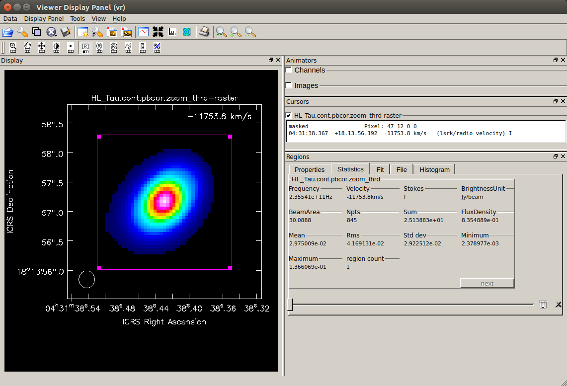 If you display the map with the 5σ threshold with
 viewer, it will look like the one on the right.
The "Total Flux" above gives the total continuum flux inside this image. To check the total flux on the
viewer, select the whole region, open the "Statistics" tab and look at the "FluxDensity" value.
Assuming that the continuum emission is thermal radiation from dust grains, and that the emission is optically thin, the dust mass
Mdust in the disk is obtained from the following equation using the continuum total flux obtained here. 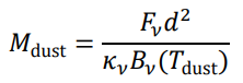
where
Fν is the total flux, d is the distance to the object, and Tdust is the dust temperature.
Bν (Tdust) represents the Planck function (black body radiation) at the dust temperature Tdust,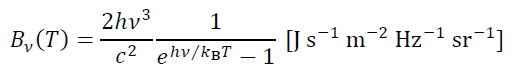
.
Also,
κν represents the dust opacity (absorption coefficient), which is assumed here as κν is approximated by the exponential function of frequency κν ∝ νβ, but β = 1 is assumed.
Note that the opacity κν, also including β, is a highly uncertain value as the properties of dust grains in disks are not well known. (Please also note that in some literature, the authors use the opacity which already assumed a gas-dust mass ratio = 100 and included the gas mass.)In this example, it is assumed that the distance to HL Tau is
d = 140 [pc] and the dust temperature is Tdust = 20 [K].
# In CASA
import math
hhh = 6.626*10**(-34) #J*s Planck constant
ccc = 2.998*10**(8) # m/s speed of light
kkb = 1.381*10**(-23) # J/K Boltzmann constant
pcc = 3.087*10**(16) #m/pc parsec
Mso = 1.989*10**(30) #kg Solar mass
J2E = 10**(-26) # 1 Jy = 10-26 W·m-2·Hz-1

# for HL Tau
dist = 140. # pc distance
Tdust = 20. # K dust temperature

imname = 'HL_Tau.cont.pbcor'
nu = imhead(imname)['refval'][2] # Hz observing frequency
Fcont = imgflx # Jy continuum flux

#Planck function
Bpf = ( (2.*hhh*nu**3) / (ccc**2) ) / ( math.exp((hhh*nu)/(kkb*Tdust))-1 )
# dust opacity (Beckwith et al. 1990)
kap = 10*((nu/(10**9))/1000) / 10# m^2 kg^-1
# dust mass (Mo)
Mdust = (Fcont*J2E*(dist*pcc)**2) / (kap*Bpf) / Mso
print(f'Dust mass on disk = {Mdust:.6f} Mo')
Dust mass on disk = 0.001313 Mo
back to top
Last Update: 2024.02.15