Participaint: Enomoto, Eleonora and Yuhang

Today we did the filter cavity green reflection characterization again after achieved its lock. Here I want to put some information we found for the green reflection from filter cavity.

Firstly let's review the set up. The configuration is we put a BS for filter cavity green reflection extracted from Faraday isolator. Small part of green goes to FC locking. Another part is used for our characterization and it is sent to a good height by using a periscope. Then let's look at some information:

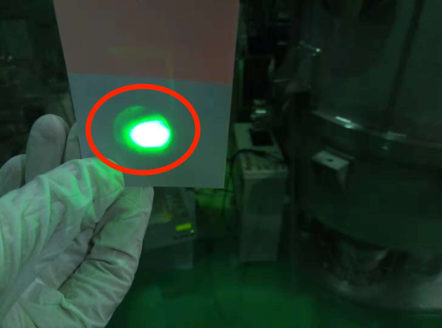
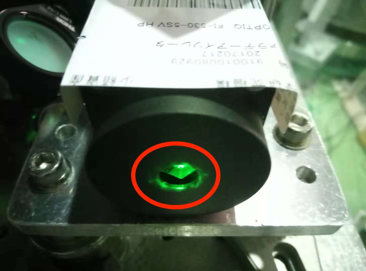
1. The reflection seems to be cutted by something if you look at our green at a decent distance. See attached figure 1. It is taken several months ago by me and Marc. As you can see, there is a very clear boundary around the green light. Although the brightest part is smaller than this boundary, it is essential to know where it is cutted. And we confirmed that it is cutted by one side of Faraday isolator whose cover is not dismounted.(See attached figure 2)

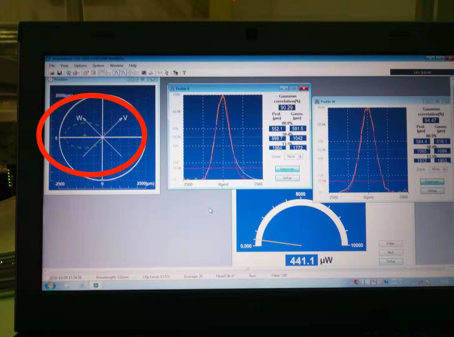
2. The reflected beam shape is quite bad. I think you have already noticed that in the attached figure 1, the beam seems to be flatted by astigmatism. This effect becomes quite obvious if you look at the beam detected by the beam profiler. See attached figure 3, the beam shape is really horizental oriented ellipse. However, the axises of our beam profiler detection is accidently aligned to two direction that have the same dimension. That means we cannot have a numerical estimation of this astigmatism by chance. But this brings also an advantage, it is roughly the average of the long axis and short axis of this ellipse. So it is reasonable to continue the measurement even in this case.

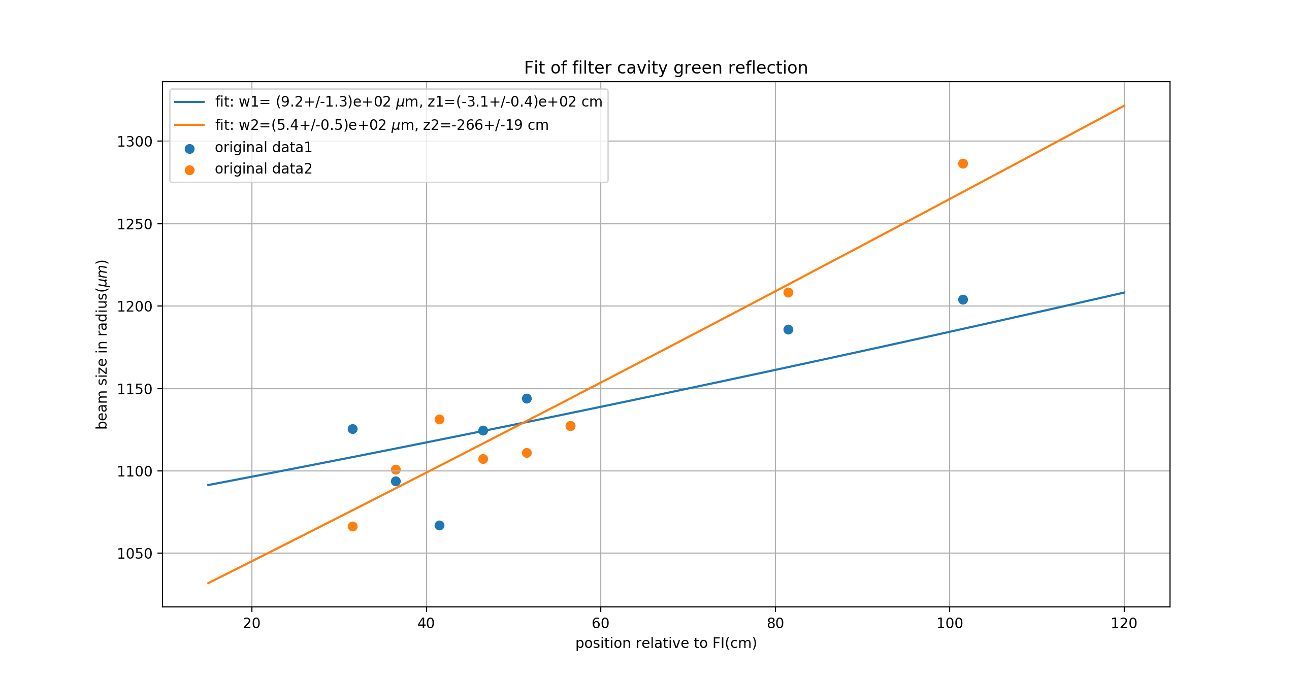
3. We did the measurement and fit of this beam directly although it is quite collimated. Besides, this beam is quite unstable. So you can see the points we took are quite scattered. Then we did the fit and the result is shown in attached figure 4. As you can see, the beam waist size is quite different in these two cases(900 and 500 um with an error of roughly 10 percent). Also the waist position has a quite large difference(-300 and -260 cm with an error of roughly 10 percent). 

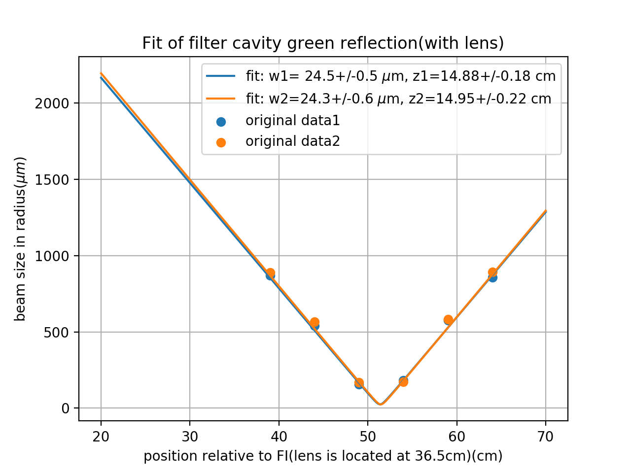
4. The last method we tried is to put a lens and do beam characterization after lens. By this characterization result, we propagate back to the beam before lens by using JaMmt and ABCD matix. However, this time we set up the average inside beam profiler as 20 while last time it is 5. Now the number we can read becomes more stable. Then we took this more stable data and did the fit. The result is shown in attached figure 5. 

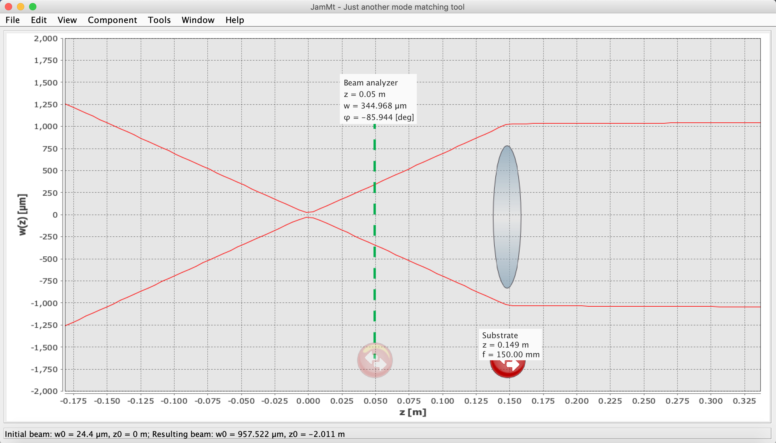
The lens we used is 150mm, and the measured result is quite reasonble now. As you can see in figure 5, z0 is both roughly 150mm. Then we used JaMmt propagate the beam back, the result is shown in attached figure 6. From this result, we can see the beam waist size should be 957um, while its position is after the lens about 2m. This means the waist is located not inside the beam going to filter cavity. Besides, there maybe a measurement shift of several millimeters of waist position of the beam after lens. And this can influence quite a lot the waist position. Also the focal lens of our 150mm lens can also be smaller or larger than this nominal 150mm value. Then influence this waist position quite a lot. But anyway, the waist position is not so important for a collamited beam. So it should be fine.

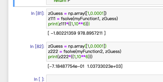
We also verify this result by using ABCD matrix. The method I used is taking the q factor of gaussian beam. Then the free space propagation is just an addation of this distance to this q. The lens is just a modification of the invert of q by 1/f. Since we use a converging lens, the f is positive. We used the detection beam wait size and waist position to reconstruct the original waist size and its position. Then make real and imaginary part equal with each other to have two equations and solve two unkown valuables. The result is shown in attached figure 7. The averange of these two result is 1.2m before the lens and wasit size is 1008um. It complies with the result of JaMmt, and this is reasonable because they are using the same principle. (Actually I want to propagate the error of fit result, but the python code of this error propagation cannot deal with imaginary number and solve equation, so I give up the error estimate in the end.)